Code: MATLAB · Python · Julia · R

# MATLAB code to generate a geometric sequence
p = 1/2;
n = 1:10;
X = p.^n;
bar(n,X,'FaceColor',[0.8, 0.2,0.2]);

# Python code to generate a geometric sequence
import numpy as np
import matplotlib.pyplot as plt
p = 1/2
n = np.arange(1,10)
X = np.power(p,n)
plt.bar(n,X)

# Julia code to generate a geometric series
using StatsPlots:bar
p = 0.5
n = 1:10
X = p .^ n
bar(n, X, legend=false)

# R code to generate a geometric series
p <- 1/2
n <- seq(1, 10)
X <- p^n
barplot(X, names.arg=1:10)

# MATLAB code to compute (N choose K) and K!
n = 10;
k = 2;
nchoosek(n,k)
factorial(k)

# Python code to compute (N choose K) and K!
from scipy.special import comb, factorial
n = 10
k = 2
comb(n, k)
factorial(k)

# Julia code to compute (N choose K) and K!
n = 10
k = 2
binomial(n, k)
factorial(k)

# R code to compute (N choose K) and K!
n <- 10
k <- 2
choose(n,k)
factorial(k)

# MATLAB code to perform an inner product
x = [1 0 -1]';
y = [3 2 0]';
z = x'*y;

# Python code to perform an inner product
import numpy as np
x = np.array([1,0,-1])
y = np.array([3,2,0])
z = np.dot(x,y) 
print(z)

# Julia code to perform an inner product
x = [1, 0, -1]
y = [3, 2, 0]
x'y

# R code to perform an inner product
x <- c(1,0,-1)
y <- c(3,2,0)
z <- t(x) %*% y
print(z)

# MATLAB code to compute the norm
x = [1 0 -1];
x_norm = norm(x);

# Python code to compute the norm
import numpy as np
x = np.array([1,0,-1])
x_norm = np.linalg.norm(x)

# Julia code to compute the norm
using LinearAlgebra:norm
x = [1, 0, -1]
norm(x)

# R code to compute the norm
x <- c(1,0,-1)
x_norm <- norm(x, type = "2")
# "2" specifies the “spectral” or 2-norm, which is the largest singular value of x
print(x_norm)

# MATLAB code to compute the weighted norm
W = [1 2 3; 4 5 6; 7 8 9];
x = [2; -1; 1];
z = x'*W*x

# Python code to compute the weighted norm
import numpy as np
W = np.array([[1, 2, 3], [4, 5, 6], [7, 8, 9]])
x = np.array([[2],[-1],[1]])
z = np.dot(x.T, np.dot(W,x))
print(z)

# Julia code to compute the weighted norm
W = [1. 2. 3.; 4. 5. 6.; 7. 8. 9.]
x = [2, -1, 1]
z = x'W*x

# R code to compute the weighted norm
W <- matrix(1:9, ncol = 3, nrow = 3)
x <- matrix(c(2,-1,1))
z <- t(x) %*% (W %*% x)
print(z)

# MATLAB code to compute a matrix inverse
X = [1 3; -2 7; 0 1]
XtXinv = inv(X'X)

# Python code to compute a matrix inverse
import numpy as np
X      = np.array([[1, 3], [-2, 7], [0, 1]])
XtX    = np.dot(X.T, X)
XtXinv = np.linalg.inv(XtX)
print(XtXinv)

# Julia code to compute a matrix inverse
X = [1 3; -2 7; 0 1]
XtXinv = inv(X'X)

# R code to compute a matrix inverse
X <- matrix(c(1,-2,0,3,7,1), nrow = 3, ncol = 2)
XtX <- t(X) %*% X
Xtxinv <- solve(XtX)
print(Xtxinv)

# MATLAB code to solve X beta = y
X      = [1 3; -2 7; 0 1];
y      = [2; 1; 0];
beta   = X\y;

# Python code to solve X beta = y
import numpy as np
X      = np.array([[1, 3], [-2, 7], [0, 1]])
y      = np.array([[2],[1],[0]])
beta   = np.linalg.lstsq(X, y, rcond=None)[0]
print(beta)

# Julia code to solve X beta = y
X = [1. 3.; -2. 7.; 0. 1.]
y = [2., 1., 0.]
beta = X\y

# R code to solve X beta = y
X <- matrix(c(1,-2,0,3,7,1), nrow = 3, ncol = 2)
y <- matrix(c(2,1,0))
beta <- solve(qr(X), y)
print(beta)

% MATLAB code to generate the histogram
load('ch3_data_English');
bar(f/100,'FaceColor',[0.9,0.6,0.0]);
xticklabels({'a','b','c','d','e','f','g','h','i','j','k','l',...
    'm','n','o','p','q','r','s','t','u','v','w','x','y','z'});
xticks(1:26);
yticks(0:0.02:0.2);
axis([1 26 0 0.13]);

# Python code generate the histogram
import numpy as np
import matplotlib.pyplot as plt
f = np.loadtxt('./ch3_data_english.txt')
n = np.arange(26)
plt.bar(n, f/100)
ntag = ['a','b','c','d','e','f','g','h','i','j','k','l','m',\
    'n','o','p','q','r','s','t','u','v','w','x','y','z']
plt.xticks(n, ntag)
plt.show()

# Julia code generate the histogram
using Plots,DelimitedFiles
f = readdlm("ch3_data_english.txt")
bar(f/100,xticks = (1:26,'a':'z'),yticks = 0.0:0.02:0.1,label = false)

# R code generate the histogram

f <- read.table('./ch3_data_english.txt')
f <- f/100
n <- c(1:26)
ntag <- c('a','b','c','d','e','f','g','h','i','j','k','l','m',
    'n','o','p','q','r','s','t','u','v','w','x','y','z')

f$index <- n
f$labels <- ntag

barplot(f$V1~f$index, xaxt = 'n', xlab = "Letters", ylab = "Values") 
axis(1, at=1:26, labels=ntag)

% MATLAB code to generate the histogram
x = [1 2 3 4 5 6];
q = randi(6,100,1);
[num,val] = hist(q,x-0.5);
bar(num/100,'FaceColor',[0.8, 0.8,0.8]);
axis([0 7 0 0.24]);

# Python code generate the histogram
import numpy as np
import matplotlib.pyplot as plt
q = np.random.randint(7,size=100)
plt.hist(q+0.5,bins=6)
plt.show()

# Julia code generate the histogram
using Plots,Random
q = rand(1:6,100)
histogram(q,bins = 6,normalize = true,label = "N = 100")

# R code generate the histogram
q <- sample(1:6, 100, replace = T)
hist(q + 0.5, 6)

% MATLAB code used to generate the plots
lambda = 1;
k      = 1000;
X      = exprnd(1/lambda,[k,1]);
[num,val] = hist(X,200);
bar(val,num,'FaceColor',[1, 0.5,0.5]);

# Python code used to generate the plots
import numpy as np
import matplotlib.pyplot as plt
lambd = 1
k = 1000
X = np.random.exponential(1/lambd, size=k)
plt.hist(X,bins=200);
plt.show()

# Julia code used to generate the plots
using Plots,Random,Distributions
lambda = 1
X = rand(Exponential(1/lambda),1_000)
histogram(X,bins = 200,label = "K = 200")

# R code used to generate the plots
lambda <- 1
k <- 1000
X <- rexp(k, rate=lambda)
hist(X, 200)

% MATLAB code to perform the cross validation
lambda = 1;
n = 1000;
X = exprnd(1/lambda,[n,1]);
m = 6:200;
J = zeros(1,195);

for i=1:195
    [num,binc] = hist(X,m(i));
    h = n/m(i);
    J(i) = 2/((n-1)*h)-((n+1)/((n-1)*h))*sum( (num/n).^2 );
end

plot(m,J,'LineWidth',4,'Color',[0.9,0.2,0.0]);

# Python code to perform the cross validation
import numpy as np
import matplotlib.pyplot as plt
lambd = 1
n     = 1000
X     = np.random.exponential(1/lambd, size=n)
m     = np.arange(5,200)
J     = np.zeros((195))

for i in range(0,195):
  hist,bins = np.histogram(X,bins=m[i])
  h = n/m[i]
  J[i] = 2/((n-1)*h)-((n+1)/((n-1)*h))*np.sum((hist/n)**2)

plt.plot(m,J);

# Julia code to perform the cross validation

using Plots,Random,Distributions,StatsBase
lambda = 1
n = 1_000
X = rand(Exponential(1/lambda),n)
m = 6:200
J = zeros(195)
for i = 1:195
    hist = fit(Histogram,X,range(minimum(X),maximum(X),length = m[i]+1))
    h = n/m[i]
    J[i] = 2/((n-1)*h)-((n+1)/((n-1)*h))*sum( (hist.weights/n).^2 )
end

plot(m,J,label = false)

# R code to perform the cross validation
lambda <- 1
n <- 1000
X <- rexp(n, rate=lambda)
m <- 6:200
J <- numeric(195)
for (i in 1:195) {
    num <- hist(X, breaks=seq(0, max(X), l=m[i]), plot=FALSE)$counts
    h <- n/m[i]
    J[i] = 2/((n-1)*h)-((n+1)/((n-1)*h))*sum((num/n)^2) 
}
plot(m, J, type="l", lwd=3)

% MATLAB code to compute the mean of a dataset
X  = rand(10000,1);
mX = mean(X);

# Python code to compute the mean of a dataset
import numpy as np
X  = np.random.rand(10000)
mX = np.mean(X)

# Julia code to compute the mean of a dataset
using Random,Statistics
X = rand(10_000)
mean(X)

# R code to compute the mean of a dataset
X <- runif(n=10000, min=0, max=1)
print(mean(X))

% MATLAB code to compute the expectation
p = [0.25 0.5 0.25];
x = [0 1 2];
EX = sum(p.*x);

# Python code to compute the expectation
import numpy as np
p = np.array([0.25, 0.5, 0.25])
x = np.array([0, 1, 2])
EX = np.sum(p*x)

# Julia code to compute the expectation
p = [0.25,0.5,0.25]
x = [0,1,2]
EX = sum(p .* x)

# R code to compute the expectation
p = c(0.25, 0.5, 0.25)
x = c(0, 1, 2)
EX = sum(p*x)
print(EX)

% MATLAB code to compute the expectation
k = 1:100;
p = 0.5.^k;
EX = sum(p.*k);

# Python code to compute the expectation
import numpy as np
k = np.arange(100)
p = np.power(0.5,k)
EX = np.sum(p*k)

# Julia code to compute the expectation
k = 1:100
p = 0.5.^k
EX = sum(p .* k)

# R code to compute the expectation
k = c(1:100)
p = 0.5 ^ k
EX = sum(p*k)
print(EX)

% MATLAB code to generate 1000 Bernoulli random variables
p = 0.5;
n = 1;
X = binornd(n,p,[1000,1]);
[num, ~] = hist(X, 10);
bar(linspace(0,1,10), num,'FaceColor',[0.4, 0.4, 0.8]);

# Python code to generate 1000 Bernoulli random variables
import numpy as np
import matplotlib.pyplot as plt
p = 0.5
n = 1
X = np.random.binomial(n,p,size=1000)
plt.hist(X,bins='auto')

# Julia code to generate 1000 Bernoulli random variables
using Plots,Distributions
p = 0.5
n = 1
X = rand(Binomial(n,p),1_000)
histogram(X,bins = 2,label = false)

# R code to generate 1000 Bernoulli random variables
p <- 0.5
n <- 1
X <- rbinom(1000, n, p)
hist(X)

% MATLAB code to generate Erdos Renyi Graph
A = rand(40,40)<0.3;
A = triu(A,1);
A = A+A';
figure(1);
G = graph(A);
plot(G, 'LineWidth', 2, 'EdgeColor', [0.1 0.6 0], 'MarkerSize',10);
set(gcf, 'Position', [100, 100, 300, 300]);
title('p = 0.3');

# Python code to generate Erdos Renyi Graph
import numpy as np
import matplotlib.pyplot as plt
import networkx as nx
A = np.random.rand(40, 40) < 0.3
A = np.triu(A, 1)
A = A + A.T
G = nx.convert_matrix.from_numpy_matrix(A)
fig, ax = plt.subplots()
nx.draw(G, with_labels=True, ax=ax)
limits = plt.axis("on")
ax.tick_params(left=True, bottom=True, labelleft=True, labelbottom=True)
plt.show()

# Julia code to generate Erdos Renyi Graph
using Plots,Random,LinearAlgebra,GraphRecipes
A = rand(40,40) .< 0.1
A = triu(A,1)
A = A + A'
graphplot(A)

# R code to generate Erdos Renyi Graph
library(igraph)
A <- matrix(runif(40*40), 40, 40) < 0.3
A[lower.tri(A, diag=TRUE)] <- FALSE
A <- A | t(A)
G <- graph_from_adjacency_matrix(A, mode="undirected")
plot(G, vertex.size=8, edge.color="darkgreen", main="p = 0.3")

% MATLAB code to generate 5000 Binomial random variables
p = 0.5;
n = 10;
X = binornd(n,p,[5000,1]);
[num, ~] = hist(X, 10);
bar( num,'FaceColor',[0.4, 0.4, 0.8]);

# Python code to generate 5000 Binomial random variables
import numpy as np
import matplotlib.pyplot as plt
p = 0.5
n = 10
X = np.random.binomial(n,p,size=5000)
plt.hist(X,bins='auto');

# Julia code to generate 5000 Binomial random variables
using Plots,Distributions
p = 0.5
n = 10
X = rand(Binomial(n,p),5_000)
histogram(X,label = false)

# R code to generate 5000 Binomial random variables
p <- 0.5
n <- 10
X <- rbinom(5000, n, p)
hist(X)

% MATLAB code to plot CDF of a binomial random variable
x = 0:10;
p = 0.5;
n = 10;
F = binocdf(x,n,p);
figure; stairs(x,F,'.-','LineWidth',4,'MarkerSize',30);

# Python code to plot CDF of a binomial random variable
import numpy as np
import matplotlib.pyplot as plt
import scipy.stats as stats
p = 0.5
n = 10
rv = stats.binom(n,p)
x  = np.arange(11)
F  = rv.cdf(x)
plt.plot(x, F, 'bo', ms=10);
plt.vlines(x, 0, F, colors='b', lw=5, alpha=0.5);

# Julia code to plot CDF of a binomial random variable
using Plots,Distributions
x = 0:10
p = 0.5
n = 10
F = cdf.(Binomial(n,p),x)
plot(x,F,linetype = :steppost,label = false,markershape = :circle)

# R code to plot CDF of a binomial random variable
p <- 0.5
n <- 10
x <- 0:n
plot(x, pbinom(x, size = n, prob = p), type="h")

% MATLAB code to plot the Poisson PMF
lambda_set = [1 4 10];
for i=1:3
    lambda = lambda_set(i);
    k = 0:1:20;
    p(:,i) = lambda.^k./factorial(k).*exp(-lambda);
end
figure;
stem(k, p(:,1),'b.','LineWidth',2,'MarkerSize',30); hold on;
stem(k, p(:,2),'.','LineWidth',2,'MarkerSize',30, 'Color', [0.1 0.5 0]);
stem(k, p(:,3),'.','LineWidth',2,'MarkerSize',30, 'Color', [1 0.5 0]);
legend('\lambda = 1', '\lambda = 4', '\lambda = 10');
grid on;
set(gcf, 'Position', [100, 100, 600, 400]);
set(gca,'FontWeight','bold','fontsize',14);

% MATLAB code to plot the Poisson CDF
lambda_set = [1 4 10];
for i=1:3
    lambda = lambda_set(i);
    k = 0:1:20;
    p(:,i) = lambda.^k./factorial(k).*exp(-lambda);
end
figure;
stairs(k, cumsum(p(:,1)), 'b.-','MarkerSize',30, 'LineWidth', 2); hold on;
stairs(k, cumsum(p(:,2)), '.-','MarkerSize',30, 'Color', [0.1 0.5 0], 'LineWidth', 2);
stairs(k, cumsum(p(:,3)), '.-','MarkerSize',30, 'Color', [1 0.5 0], 'LineWidth', 2);
legend('\lambda = 1', '\lambda = 4', '\lambda = 10', 'Location', 'SE');
grid on;
set(gcf, 'Position', [100, 100, 600, 400]);
set(gca,'FontWeight','bold','fontsize',14);

# Python code to plot the Poisson PMF
import numpy as np
import matplotlib.pyplot as plt
from scipy.special import factorial
lambda_set = [1, 4, 10]
p = np.zeros((20, 3))
k = np.arange(0, 20)
for i in range(0, 3):
    lambd = lambda_set[i]
    p[:,i] = lambd**k/factorial(k)*np.exp(-lambd)

plt.plot(k, p[:,0], 'bo')
plt.vlines(k, 0 , p[:,0], colors='b', lw=2)
plt.plot(k, p[:,1], 'go')
plt.vlines(k, 0 , p[:,1], colors='g', lw=2)
plt.plot(k, p[:,2], 'yo')
plt.vlines(k, 0 , p[:,2], colors='y', lw=2)
labels = ["lambda = 1", "lambda = 4", "lambda = 10"]
plt.legend(labels=labels)
plt.grid()
plt.show()

# Python code to plot the Poisson CDF
import numpy as np
import matplotlib.pyplot as plt
from scipy.special import factorial
lambda_set = [1, 4, 10]
p = np.zeros((20, 3))
k = np.arange(0, 20)
for i in range(0, 3):
    lambd = lambda_set[i]
    p[:,i] = lambd**k/factorial(k)*np.exp(-lambd)

plt.step(k, np.cumsum(p[:,0]), 'b')
plt.step(k, np.cumsum(p[:,1]), 'g')
plt.step(k, np.cumsum(p[:,2]), 'y')
plt.plot(k, np.cumsum(p[:,0]), 'bo')
plt.plot(k, np.cumsum(p[:,1]), 'go')
plt.plot(k, np.cumsum(p[:,2]), 'yo')
labels = ["lambda = 1", "lambda = 4", "lambda = 10"]
plt.legend(labels=labels)
plt.grid()
plt.show()

# Julia Code for the Poisson PMF 
using Plots,Distributions
lambda_set = [1,4,10]
p = zeros(21,3)
k = 0:1:20
for i = 1:3
    p[:,i] = pdf.(Poisson(lambda_set[i]),k)
end
plot(k,p[:,1],line = :stem,markershape = :circle,label = "lambda = 1")
plot!(k,p[:,2],line = :stem,markershape = :circle,label = "lambda = 4")
plot!(k,p[:,3],line = :stem,markershape = :circle,label = "lambda = 10")

# Julia Code for Poisson CDF
using Plots,Distributions
lambda_set = [1,4,10]
p = zeros(21,3)
k = 0:1:20
for i = 1:3
    p[:,i] = cdf.(Poisson(lambda_set[i]),k)
end
plot(k,p[:,1],line = :steppost,markershape = :circle,label = "lambda = 1")
plot!(k,p[:,2],line = :steppost,markershape = :circle,label = "lambda = 4")
plot!(k,p[:,3],line = :steppost,markershape = :circle,label = "lambda = 10",legend = :bottomright)

# R code to plot the Poisson PMF
library(pracma)
lambda_set = c(1, 4, 10)
p = zeros(21, 3)
k = seq(0, 20)
for (i in 1:3) {
    p[,i] = dpois(k, lambda_set[i])
}

plot(k, p[,1], type='h', lwd=3, col="blue")
grid()
legend(15, 0.36, legend=c("lambda  = 1", "lambda  = 4", "lambda  = 10"), col=c("blue", "darkgreen", "orange"), lwd=3)
lines(k, p[,1], type='p', cex=2, pch=16, col="blue")
lines(k, p[,2], type='h', lwd=3, col="darkgreen")
lines(k, p[,2], type='p', cex=2, pch=16, col="darkgreen")
lines(k, p[,3], type='h', lwd=3, col="orange")
lines(k, p[,3], type='p', cex=2, pch=16, col="orange")

# R code to plot the Poisson CDF 
library(pracma)
lambda_set = c(1, 4, 10)
p = zeros(21, 3)
k = seq(0, 20)
for (i in 1:3) {
    p[,i] = ppois(k, lambda_set[i])
}

plot(k, p[,3], type='s', lwd=3, col="orange")
grid()
legend(15, 0.36, legend=c("lambda  = 1", "lambda  = 4", "lambda  = 10"), col=c("blue", "darkgreen", "orange"), lwd=3)
lines(k, p[,3], type='p', cex=2, pch=16, col="orange")
lines(k, p[,2], type='s', lwd=3, col="darkgreen")
lines(k, p[,2], type='p', cex=2, pch=16, col="darkgreen")
lines(k, p[,1], type='s', lwd=3, col="blue")
lines(k, p[,1], type='p', cex=2, pch=16, col="blue")

% MATLAB code to approximate binomial using Poisson
n = 5000;
p = 0.01;
lambda = n*p;
x = 0:120;
y = binopdf(x,n,p);
z = poisspdf(x,lambda);
stem(x,y,'Color',[0.5,0.7,0],'LineWidth', 2); hold on;
plot(x,z,'b','LineWidth',2);
legend('Binomial, n = 5000, p = 0.01','Poisson, \lambda = 50');
xlabel('k');
ylabel('Probability');
grid on;
set(gcf, 'Position', [100, 100, 800, 300]);
set(gca,'FontWeight','bold','fontsize',14);

# Python code to approximate binomial using Poisson
import numpy as np
import matplotlib.pyplot as plt
import scipy.stats as stats
n = 5000; p = 0.01
rv1 = stats.binom(n,p)
X   = rv1.rvs(size=10000)
plt.figure(1); plt.hist(X,bins=np.arange(0,100));
rv2 = stats.poisson(n*p)
f   = rv2.pmf(bin)
plt.figure(2); plt.plot(f);

# Julia code to approximate binomial using Poisson
using Plots,Distributions
n = 5_000
p = 0.01
lambda = n*p
x = 0:120
y = pdf.(Binomial(n,p),x)
z = pdf.(Poisson(lambda),x)
plot(x,y,line = :stem,markershape = :circle,label = "Binomial,n = 5000,p = 0.01")
plot!(x,z,label = "Poisson, lambda = 50")

# R code to approximate binomial using Poisson
n = 5000
p = 0.01
lambda = n*p
x = 0:120
y = dbinom(x, n, p)
z = dpois(x, lambda)

plot(x, y, lwd=2, type="h", col="darkolivegreen3", xlab="k", ylab="Probability")
legend(63, 0.053, legend=c("Binomial, n=5000, p=0.01", "Poisson, lambda = 50"), col=c("darkolivegreen3", "blue"), lwd=3)
grid()
lines(x, y, lwd=2, cex=1, type="p", col="darkolivegreen3")
lines(x, z, lwd=2, type="l", col="blue")

% MATLAB to demonstrate the photon shot noise
x = im2double(imread('cameraman.tif'));

alpha = 10;
lambda = alpha*x;
X1 = poissrnd(lambda);

alpha = 100;
lambda = alpha*x;
X2 = poissrnd(lambda);

alpha = 1000;
lambda = alpha*x;
X3 = poissrnd(lambda);

figure;
subplot(131); imshow(X1,[]); title('\alpha = 10');
subplot(132); imshow(X2,[]); title('\alpha = 100');
subplot(133); imshow(X3,[]); title('\alpha = 1000');

# Python to demonstrate the photon shot noise
import numpy as np
import matplotlib.pyplot as plt
import cv2
x = cv2.imread('cameraman.tif', 0)/255
width = len(x)

alpha = 10
lam = alpha * x
X1 = np.random.poisson(lam=lam, size=(width, width))

alpha = 100
lam = alpha * x
X2 = np.random.poisson(lam=lam, size=(width, width))

alpha = 1000
lam = alpha * x
X3 = np.random.poisson(lam=lam, size=(width, width))

plt.figure(1)
plt.imshow(X1, cmap='gray')
plt.title("alpha = 10")
plt.figure(2)
plt.imshow(X2, cmap='gray')
plt.title("alpha = 100")
plt.figure(3)
plt.imshow(X3, cmap='gray')
plt.title("alpha = 1000")
plt.show()

# Julia code to demonstrate the photon shot noise
using Distributions,Images,ImageView,Random
x = Float64.(load("cameraman.tif"))

alpha = 10
lambda = alpha*x
X1 = rand.(Poisson.(lambda))
imshow(X1)

alpha = 100
lambda = alpha*x
X1 = rand.(Poisson.(lambda))
imshow(X1)

alpha = 1_000
lambda = alpha*x
X1 = rand.(Poisson.(lambda))
imshow(X1)

# R code to demonstrate the photon shot noise 
library(imager)
x = as.data.frame(load.image("cameraman.tif"))
x = xtabs(value ~ x+y, data=x)
width = sqrt(length(x))

alpha = 10
lambda = alpha * x
X1 = rpois(length(lambda), lambda)
X1 = array(X1, c(width, width))

alpha = 100
lambda = alpha * x
X2 = rpois(length(lambda), lambda)
X2 = array(X2, c(width, width))

alpha = 1000
lambda = alpha * x
X3 = rpois(length(lambda), lambda)
X3 = array(X3, c(width, width))

# Flip matrix since `image()` reads the matrix bottom up
flip_matrix = function(m) m[,nrow(m):1]

# Plot images together
layout(matrix(1:3, 1, 3), respect=TRUE)
image(flip_matrix(X1), col=gray.colors(255), main = expression(paste(alpha, " = 10")))
image(flip_matrix(X2), col=gray.colors(255), main = expression(paste(alpha, " = 100")))
image(flip_matrix(X3), col=gray.colors(255), main = expression(paste(alpha, " = 1000")))

# MATLAB code to generate the PDF and CDF
gmm = gmdistribution([0; 5], cat(3,1,1), [0.3 0.7]);

x  = linspace(-5, 10, 1000)';
f  = pdf(gmm, x);
x1 = linspace(-5,1,1000)';
f1 = pdf(gmm,x1);
figure;
area(x1,f1,'EdgeColor','none','FaceColor',[0.8,0.8,1]);hold on;
plot(x, f, 'LineWidth', 6);
grid on;
axis([-5 10 0 0.4]);
set(gcf, 'Position', [100, 100, 600, 300]);
set(gca,'FontWeight','bold','fontsize',14);

F = cdf(gmm, x);
figure;
plot(x, F, 'LineWidth', 6);
grid on;
axis([-5 10 0 1]);
set(gcf, 'Position', [100, 100, 600, 300]);
set(gca,'FontWeight','bold','fontsize',14);

# Python code to generate the PDF and CDF
import numpy as np
import matplotlib.pyplot as plt
from scipy.stats import norm
w, mu, sd = [0.3, 0.7], [0, 5], [1, 1]
x = np.linspace(-5, 10, 1000)
f = w[0]*norm.pdf(x, mu[0], sd[0]) + w[1]*norm.pdf(x, mu[1], sd[1])
F = w[0]*norm.cdf(x, mu[0], sd[0]) + w[1]*norm.cdf(x, mu[1], sd[1])
plt.figure()
plt.fill_between(x[x <= 1], f[x <= 1], color=(0.8, 0.8, 1))
plt.plot(x, f, linewidth=6); plt.axis([-5, 10, 0, 0.4]); plt.grid(True)
plt.figure()
plt.plot(x, F, linewidth=6); plt.axis([-5, 10, 0, 1]); plt.grid(True)
plt.show()

# Julia code to generate the PDF and CDF
using Distributions
using Plots

gmm = MixtureModel(Normal[Normal(0, 1), Normal(5, 1),], [0.3, 0.7])

p1 = plot(x -> 0, -5, 1, fillrange= x->pdf(gmm, x), 
    linealpha=0, fillcolor=RGB(0.8, 0.8, 1), alpha=0.5, label=false) # style
plot!(p1, x -> pdf(gmm, x), -5, 10, 
    color=1, linewidth=6, label="PDF") # style

p2 = plot(x -> cdf(gmm, x), -5, 10, 
    linewidth=6, label="CDF")

plot(p1, p2, layout=(1, 2), 
    size=(600, 300), legend=:topleft)

# R code to generate the PDF and CDF
library(EnvStats)

x = seq(-5, 10, (5+10)/1000)
x = sort(x)
f = dnormMix(x, 0, 1, 5, 1, p.mix=c(0.7))
plot(x,f, xlim=c(-5,10), ylim=c(0,0.4), type="n")
lines(x, f, lwd=4, col="blue")
polygon(c(min(x), x[x<=0.8]), c(f[x<=0.8], 0), col="lightblue")
grid()

F = pnormMix(x, 0, 1, 5, 1, p.mix=c(0.7))
plot(x, F, type="n")
lines(x, F, lwd=4, col="blue")
grid()

# MATLAB code to generate the PDF and CDF of a uniform random variable
unif = makedist('Uniform','lower',-3,'upper',4);

x  = linspace(-5, 10, 1500)';
f  = pdf(unif, x);
x1 = linspace(-5,1,1500)';
f1 = pdf(unif,x1);
figure;
area(x1,f1,'EdgeColor','none','FaceColor',[0.8,0.8,1]);hold on;
plot(x, f, 'LineWidth', 6);
grid on;
axis([-5 10 0 0.4]);
set(gcf, 'Position', [100, 100, 600, 300]);
set(gca,'FontWeight','bold','fontsize',14);

F = cdf(unif, x);
figure;
plot(x, F, 'LineWidth', 6); hold on;
plot(x(600), F(600), 'ko', 'LineWidth', 2, 'MarkerSize', 10, 'MarkerFaceColor', [0.8,0.8,1]);
grid on;
axis([-5 10 0 1]);
set(gcf, 'Position', [100, 100, 600, 300]);
set(gca,'FontWeight','bold','fontsize',14);

# Python code to generate the PDF and CDF of a uniform random variable
import numpy as np
import matplotlib.pyplot as plt
import scipy.stats as stats
x = np.linspace(-5,10,1500)
f = stats.uniform.pdf(x,-3,4)
F = stats.uniform.cdf(x,-3,4)
plt.plot(x,f); plt.show()
plt.plot(x,F); plt.show()

# Julia code to generate the PDF and CDF of a uniform random variable
using Distributions
using Plots

u = Uniform(-3, 4)

# pdf
p1 = plot(x -> 0, -5:0.01:1, fillrange=x->pdf(u, x),
    linealpha=0, fillcolor=RGB(0.8, 0.8, 1), alpha=0.5, label=false)
plot!(p1, x -> pdf(u, x), -5, 10, 
    color=1, linewidth=6, ylims=(0, 0.4), label="PDF")

# cdf
p2 = plot(x -> cdf(u, x), -5:0.01:10, 
    linewidth=6, label="CDF")
vline!(p2, [-3, 4], 
    linestyle=:dash, color=:green, label=false)

plot(p1, p2, layout=(1, 2), 
    size=(600, 300), legend=:topleft)

# R code to generate the PDF and CDF
x = seq(-5, 10, (5+10)/1500)
f = dunif(x, -3, 4)
F = punif(x, -3, 4)
plot(x, f, type="n")
lines(x, f, lwd=5)
grid()
plot(x, F, type="n")
lines(x, F, lwd=5)
grid()

# MATLAB code to generate the PDF and CDF of an exponential random variable
pd = makedist('exp',2);

x  = linspace(-5, 10, 1500)';
f  = pdf(pd, x);
x1 = linspace(-5,1,1500)';
f1 = pdf(pd,x1);
figure;
area(x1,f1,'EdgeColor','none','FaceColor',[0.8,0.8,1]);hold on;
plot(x, f, 'LineWidth', 6);
grid on;
axis([-5 10 0 0.6]);
set(gcf, 'Position', [100, 100, 600, 300]);
set(gca,'FontWeight','bold','fontsize',14);

F = cdf(pd, x);
figure;
plot(x, F, 'LineWidth', 6); hold on;
plot(x(600), F(600), 'ko', 'LineWidth', 2, 'MarkerSize', 10, 'MarkerFaceColor', [0.8,0.8,1]);
grid on;
axis([-5 10 0 1]);
set(gcf, 'Position', [100, 100, 600, 300]);
set(gca,'FontWeight','bold','fontsize',14);

# Python code to generate the PDF and CDF
import numpy as np
import matplotlib.pyplot as plt
import scipy.stats as stats
x = np.linspace(-5,10,1500)
f = stats.expon.pdf(x,2)
F = stats.expon.cdf(x,2)
plt.plot(x,f); plt.show()
plt.plot(x,F); plt.show()

# Julia code to generate the PDF and CDF of an exponential random variable
using Distributions
using Plots

u = Exponential(2)

# pdf
p1 = plot(x -> 0, -5:0.01:1, fillrange=x->pdf(u, x),
    linealpha=0, fillcolor=RGB(0.8, 0.8, 1), alpha=0.5, label=false)
plot!(p1, x -> pdf(u, x), -5, 10, 
    color=1, linewidth=6, ylims=(0, 0.6), label="PDF")

# cdf
p2 = plot(x -> cdf(u, x), -5:0.01:10, 
    linewidth=6, label="CDF")

plot(p1, p2, layout=(1, 2), 
    size=(600, 300), legend=:topleft)

# R code to generate the PDF and CDF
x = seq(-5, 10, (5+10)/1500)
f = dexp(x, 1/2)
F = pexp(x, 1/2)
# PDF
plot(x, f, type="n")
lines(x, f, lwd=5, col="blue")
grid()

# CDF
plot(x, F, type="n")
lines(x, F, lwd=5, col="blue")
grid()

# MATLAB code to generate 1000 uniform random numbers
a = 0; b = 1;
X = unifrnd(a,b,[1000,1]);
hist(X);

# Python code to generate 1000 uniform random numbers
import scipy.stats as stats
a = 0; b = 1;
X = stats.uniform.rvs(a,b,size=1000)
plt.hist(X);

# Julia code to generate 1000 uniform random numbers
using Distributions
using Plots

u = Uniform(0, 1) # same as Uniform()
X = rand(u, 1000)
histogram(X)

# R code to generate 1000 uniform random numbers
a = 0; b = 1;
X = runif(1000, a, b)
hist(X)
grid()

# MATLAB code to compute empirical mean, var, median, mode
X = unifrnd(a,b,[1000,1]);
M = mean(X);
V = var(X);
Med = median(X);
Mod = mode(X);

# Python code to compute empirical mean, var, median, mode
X = stats.uniform.rvs(a,b,size=1000)
M = np.mean(X)
V = np.var(X)
Med = np.median(X)
Mod = stats.mode(X)

# Julia code to compute empirical mean, var, median, mode
using Distributions
u = Uniform(0, 1)
X = rand(u, 1000)

M = mean(X)
V = var(X)
Med = median(X)
Mod = mode(X)

# R code to computer empirical mean, var, median, mode
library(pracma)
a = 0; b = 1;
X = runif(1000, a, b)
M = mean(X)
V = var(X)
Med = median(X)
Mod = Mode(X)

# MATLAB code to compute the probability P(0.2 < X < 0.3)
a = 0; b = 1;
F = unifcdf(0.3,a,b) - unifcdf(0.2,a,b)

# Python code to compute the probability P(0.2 < X < 0.3)
import scipy.stats as stats
a = 0; b = 1;
F = stats.uniform.cdf(0.3,a,b)-stats.uniform.cdf(0.2,a,b)

# Julia code to compute the probability P(0.2 < X < 0.3)
using Distributions

u = Uniform(0, 1)
F = cdf(u, 0.3) - cdf(u, 0.2)

# R code to compute the probability P(0.2 < X < 0.3)
a = 0; b = 1;
F = punif(0.3, a, b) - punif(0.2, a, b)

# MATLAB code to generate PDF and CDF of an exponential random variable
lambda1 = 1/2;
lambda2 = 1/5;

x = linspace(0,1,1000);
f1 = pdf('exp',x, lambda1);
f2 = pdf('exp',x, lambda2);

figure(1);
plot(x, f1, '-.', 'LineWidth', 4, 'Color', [0 0.2 0.8]); hold on;
plot(x, f2, 'LineWidth', 4, 'Color', [0.8 0.2 0]);
axis([0 1 0 6]);
legend('\lambda = 2', '\lambda = 5','Location','NE');
grid on;
set(gcf, 'Position', [100, 100, 600, 400]);
set(gca,'FontWeight','bold','fontsize',14);

F1 = cdf('exp',x, lambda1);
F2 = cdf('exp',x, lambda2);
figure(2);
plot(x, F1, '-.', 'LineWidth', 4, 'Color', [0 0.2 0.8]); hold on;
plot(x, F2, 'LineWidth', 4, 'Color', [0.8 0.2 0]);
axis([0 1 0 1.2]);
legend('\lambda = 2', '\lambda = 5','Location','SE');
grid on;
set(gcf, 'Position', [100, 100, 600, 400]);
set(gca,'FontWeight','bold','fontsize',14);

# Python code to generate PDF and CDF of an exponential random variable
lambd1 = 1/2
lambd2 = 1/5
x = np.linspace(0,1,1000)
f1 = stats.expon.pdf(x,scale=lambd1)
f2 = stats.expon.pdf(x,scale=lambd2)
plt.plot(x, f1)
plt.plot(x, f2)

F1 = stats.expon.cdf(x,scale=lambd1)
F2 = stats.expon.cdf(x,scale=lambd2)
plt.plot(x, F1)
plt.plot(x, F2)

# Julia code to generate PDF and CDF of an exponential random variable
using Distributions 
using Plots

exp1 = Exponential(1/2)
exp2 = Exponential(1/5)

# Plotting the pdfs
p1 = plot(x -> pdf(exp1, x), 0, 1, 
    linewidth=4, linestyle=:dashdot, color=RGB(0,0.2,0.8), label="lambda = 2")
plot!(p1, x -> pdf(exp2, x), 0, 1,
    linewidth=4, color=RGB(0.8,0.2,0), label="lambda = 5")

# Plotting the cdfs
p2 = plot(x -> cdf(exp1, x), 0, 1, 
    linewidth=4, linestyle=:dashdot, color=RGB(0,0.2,0.8), label="lambda = 2", legend=:topleft)
plot!(p2, x -> cdf(exp2, x), 0, 1,
    linewidth=4, color=RGB(0.8,0.2,0), label="lambda = 5")

# Figure with both plots
plot(p1, p2, layout=(1, 2), 
    size=(600, 400))

# R code to generate the PDF and CDF of an exponential random variable
lambda1 = 1/2
lambda2 = 1/5
x = seq(0, 1, (0+1)/1000)
f1 = dexp(x, 1/lambda1)
f2 = dexp(x, 1/lambda2)
plot(x, f2, type="n")
lines(x, f1, lwd=4, col="blue")
lines(x, f2, lwd=4, col="red")
legend(0, 1, legend=c(expression(paste(lambda, "=5")), expression(paste(lambda, "=2"))), col=c("red", "blue"), lty=1:1)
grid()

F1 = pexp(x, 1/lambda1)
F2 = pexp(x, 1/lambda2)
plot(x, F2, type="n")
lines(x, F1, lwd=4, col="blue")
lines(x, F2, lwd=4, col="red")
legend(0, 1, legend=c(expression(paste(lambda, "=5")), expression(paste(lambda, "=2"))), col=c("red", "blue"), lty=1:1)
grid()

# MATLAB code to generate standard Gaussian PDF and CDF
x = linspace(-5,5,1000);
f = normpdf(x,0,1);

x1 = linspace(-5,-1,1000);
f1 = normpdf(x1,0,1);

area(x1,f1,'EdgeColor','none','FaceColor',[0.8,0.8,0.8]);hold on;
plot(x,f,'LineWidth',6,'Color',[0,0,0]);
grid on;
xticks(-5:1:5);
yticks(0:0.1:0.5);
set(gcf, 'Position', [100, 100, 600, 300]);
set(gca,'FontWeight','bold','fontsize',18);
axis([-5 5 0 0.5]);

figure;
F = normcdf(x,0,1);
plot(x,F,'LineWidth',6,'Color',[0,0,0]); hold on;
plot(x(401), F(401), 'ko', 'LineWidth', 2, 'MarkerSize', 15, 'MarkerFaceColor', [0.8 0.8 0.8]);
grid on;
xticks(-5:1:5);
yticks(0:0.2:1);
set(gcf, 'Position', [100, 100, 600, 300]);
set(gca,'FontWeight','bold','fontsize',18);
axis([-5 5 0 1]);

# Python code to generate standard Gaussian PDF and CDF
import numpy as np
import matplotlib.pyplot as plt
import scipy.stats as stats
x = np.linspace(-10,10,1000)
f = stats.norm.pdf(x)
F = stats.norm.cdf(x)
plt.plot(x,f); plt.show()
plt.plot(x,F); plt.show()

# Julia code to generate standard Gaussian PDF and CDF
using Distributions
using Plots

normdist = Normal()

p1 = plot(x -> 0, -5:0.01:-1, fillrange=x->pdf(normdist, x),
    linealpha=0, fillcolor=RGB(0.8, 0.8, 1), alpha=0.5, label=false)
plot!(p1, x -> pdf(normdist, x), -5, 5, 
    color=1, linewidth=6, ylims=(0, 0.6), label="PDF")

p2 = plot(x -> cdf(normdist, x), -5:0.01:5, 
    linewidth=6, label="CDF")

plot(p1, p2, layout=(1, 2), 
    size=(600, 300), legend=:topleft)

# R code to generate a Gaussian PDF
x = seq(-10, 10, (10+10)/1000)
mu = 0; sigma = 1;
f = dnorm(x, mu, sigma)
plot(x, f, type="n")
lines(x, f, lwd=4, col="blue")
grid()

# R code to generate standard Gaussian PDF and CDF
x = seq(-5, 5, (5+5)/1000)
f = dnorm(x)
F = pnorm(x)
plot(x, f, type = "n")
lines(x, f, lwd=6)
grid()
plot(x, F, type = "n")
lines(x, F, lwd=6)
grid()

# MATLAB code to plot a Gamma distribution
x = linspace(0,30,1000);
theta = 1;
plot(x,gampdf(x,2,theta),'LineWidth',4, 'Color',[0 0 0]); hold on;
plot(x,gampdf(x,5,theta),'LineWidth',4, 'Color',[0.2 0.2 0.2]); 
plot(x,gampdf(x,10,theta),'LineWidth',4, 'Color',[0.4 0.4 0.4]);
plot(x,gampdf(x,15,theta),'LineWidth',4, 'Color',[0.6 0.6 0.6]);
plot(x,gampdf(x,20,theta),'LineWidth',4, 'Color',[0.8 0.8 0.8]); hold off;
legend('k = 2', 'k = 5', 'k = 10', 'k = 15', 'k = 20', 'Location', 'NE');
grid on;
set(gcf, 'Position', [100, 100, 600, 300]);
set(gca,'FontWeight','bold','fontsize',14);

# MATLAB code to compute skewness and kurtosis
X = random('gamma',3,5,[10000,1]);
s = skewness(X);
k = kurtosis(X);

# Python code to compute skewness and kurtosis
import scipy.stats as stats
X = stats.gamma.rvs(3,5,size=10000)
s = stats.skew(X)
k = stats.kurtosis(X)

# Julia code to plot a Gamma distribution
using Distributions
using Plots

theta = 1

p1 = plot(size=(600, 300))
plot!(p1, x -> pdf(Gamma(2, theta), x), 0, 30, lw=4, c=RGB(0,0,0), label="k = 2")
plot!(p1, x -> pdf(Gamma(5, theta), x), 0, 30, lw=4, c=RGB(0.2,0.2,0.2), label="k = 5")
plot!(p1, x -> pdf(Gamma(10, theta), x), 0, 30, lw=4, c=RGB(0.4,0.4,0.4), label="k = 10")
plot!(p1, x -> pdf(Gamma(15, theta), x), 0, 30, lw=4, c=RGB(0.6,0.6,0.6), label="k = 15")
plot!(p1, x -> pdf(Gamma(20, theta), x), 0, 30, lw=4, c=RGB(0.8,0.8,0.8), label="k = 20")

# Julia code to compute skewness and kurtosis
X = rand(Gamma(3, 5), 10_000)
s = skewness(X)
k = kurtosis(X)

# R code to plot a Gamma distribution
x = seq(0, 30, (0+30)/1000)
theta = 1
plot(x, dgamma(x, 2, theta), type = "n")
lines(x, dgamma(x, 2, theta), lwd = 4)
lines(x, dgamma(x, 5, theta), lwd = 4, col = "#333333")
lines(x, dgamma(x, 10, theta), lwd = 4, col = "#666666")
lines(x, dgamma(x, 15, theta), lwd = 4, col = "#999999")
lines(x, dgamma(x, 20, theta), lwd = 4, col = "#CCCCCC")
legend(23, 0.36, legend=c("k = 2", "k = 5", "k = 10", "k = 15", "k = 20"), col=c("1", "#333333", "#666666", "#999999", "#CCCCCC"), lwd = 4,lty=1:1)
grid()

library(e1071)
X = rgamma(10000, 3, 5)
s = skewness(X)
k = kurtosis(X)

# MATLAB code to generate Gaussian from uniform
mu    = 3;
sigma = 2;
U  = rand(10000,1);
gU = sigma*icdf('norm',U,0,1)+mu;
[num,val] = hist(U,30);
figure; bar(val,num,'FaceColor',[0.8, 0.8,0.8]);
set(gcf, 'Position', [100, 100, 600, 400]); grid on;
set(gca,'FontWeight','bold','fontsize',14);

[num,val] = hist(gU,30);
figure; bar(val,num,'FaceColor',[1, 0.8, 0]);
set(gcf, 'Position', [100, 100, 600, 400]); grid on;
set(gca,'FontWeight','bold','fontsize',14);

# Python code to generate Gaussian from uniform
import numpy as np
import matplotlib.pyplot as plt
import scipy.stats as stats

mu = 3
sigma = 2
U  = stats.uniform.rvs(0,1,size=10000)
gU = sigma*stats.norm.ppf(U)+mu
plt.hist(U); plt.show()
plt.hist(gU); plt.show()

# Julia code to generate Gaussian from uniform
using Distributions
using Plots

mu = 3
sigma = 2
U = rand(10_000)
gU = sigma * quantile(Normal(), U) .+ mu

p1 = histogram(U, label="U")
p2 = histogram(gU, label="gU")
plot(p1, p2, layout=(1, 2), size=(600, 300), legend=:topleft)

# R code to generate Gaussian from uniform
library(HDInterval)
mu = 3
sigma = 2
U = runif(10000, 0, 1)
gU = sigma * inverseCDF(U, pnorm) + mu;
hist(U)
grid()

hist(gU, col="yellow")
grid()

% MATLAB code to visualize correlation coefficients
x = mvnrnd([0,0],[3 1; 1 1],1000);
% x = mvnrnd([0,0],[3 0; 0 3],1000);
% x = mvnrnd([0,0],[3 2.9; 2.9 3],1000);
s = scatter(x(:,1),x(:,2),60);
s.LineWidth = 1;
s.MarkerEdgeColor = [0 0.2 0.6];
s.MarkerFaceColor = [0.9 0.5 0];
axis([-5 5 -5 5]);
xticks(-5:5);
yticks(-5:5);
set(gcf, 'Position', [100, 100, 400, 400]);
set(gca,'FontWeight','bold','fontsize',14);
std1 = std(x(:,1));
std2 = std(x(:,2));
m1   = mean(x(:,1));
m2   = mean(x(:,2));
Exy  = mean(x(:,1).*x(:,2));
r    = (Exy-m1*m2)/(std1*std2);

# Python code to compute the correlation coefficient
import numpy as np
import scipy.stats as stats
import matplotlib.pyplot as plt
x = stats.multivariate_normal.rvs([0,0], [[3,1],[1,1]], 10000)
plt.figure(); plt.scatter(x[:,0],x[:,1])
rho,_ = stats.pearsonr(x[:,0],x[:,1])
print(rho)

# Julia code to compute the correlation coefficient
using Distributions
using Plots

x = rand(MvNormal([0, 0], [3 1; 1 1]), 1000)
# x = rand(MvNormal([0, 0], [3 0; 0 3]), 1000)
# x = rand(MvNormal([0, 0], [3 2.9; 2.9 3]), 1000)
scatter(x[1, :], x[2, :])

sigma1 = std(x[1, :])
sigma2 = std(x[2, :])
mu1 = mean(x[1, :])
mu2 = mean(x[2, :])
Exy = mean(x[1, :] .* x[2, :])
rho = (Exy - mu1 * mu2) / (sigma1 * sigma2)

# R code to visualize correlation coefficients
install.packages("MASS")
library(MASS)

x <- mvrnorm(mu=c(0,0),Sigma=matrix(c(3,1,1,1), 2,2),n=10000)
plot(x[,1], x[,2])
rho = cor(x[,1], x[,2], method=c('pearson'))
print(rho)

% MATLAB code to compute a mean vector
X    = randn(100,2);
mX   = mean(X,2);

# Python code to compute a mean vector
import numpy as np
import scipy.stats as stats
X = stats.multivariate_normal.rvs([0,0],[[1,0],[0,1]],100)
mX = np.mean(X,axis=1)

# Julia code to compute a mean vector.
using Statistics
X = randn(100, 2)
mean(X, dims=1)

# R code to compute a mean vector
x <- mvrnorm(mu=c(0,0),Sigma=matrix(c(1,0,0,1), 2,2),n=100)
mX <- colMeans(x)

% MATLAB code to compute covariance matrix
X    = randn(100,2);
covX = cov(X);

# Python code to compute covariance matrix
import numpy as np
import scipy.stats as stats
X = stats.multivariate_normal.rvs([0,0],[[1,0],[0,1]],100)
covX = np.cov(X,rowvar=False)
print(covX)

# Julia code to compute covariance matrix.
using Statistics
X = randn(100, 2)
cov(X)

# R code to compute covariance matrix.
x <- mvrnorm(mu=c(0,0),Sigma=matrix(c(1,0,0,1), 2,2),n=100)
covX <- cov(x)
print(covX)

% MATLAB code: Overlay random numbers with the Gaussian contour.
X  = mvnrnd([0 0],[.25 .3; .3 1],1000);
x1 = -2.5:.01:2.5;
x2 = -3.5:.01:3.5;
[X1,X2] = meshgrid(x1,x2);
F = mvnpdf([X1(:) X2(:)],[0 0],[.25 .3; .3 1]);
F = reshape(F,length(x2),length(x1));

figure(1);
scatter(x(:,1),x(:,2),'rx', 'LineWidth', 1.5); hold on;
contour(x1,x2,F,[.001 .01 .05:.1:.95 .99 .999], 'LineWidth', 2);

# Python code: Overlay random numbers with the Gaussian contour.
import numpy as np
import scipy.stats as stats
import matplotlib.pyplot as plt

X = stats.multivariate_normal.rvs([0,0],[[0.25,0.3],[0.3,1.0]],1000)
x1 = np.arange(-2.5, 2.5, 0.01)
x2 = np.arange(-3.5, 3.5, 0.01)
X1, X2 = np.meshgrid(x1,x2)
Xpos = np.empty(X1.shape + (2,))
Xpos[:,:,0] = X1
Xpos[:,:,1] = X2

F = stats.multivariate_normal.pdf(Xpos,[0,0],[[0.25,0.3],[0.3,1.0]])

plt.scatter(X[:,0],X[:,1])
plt.contour(x1,x2,F)

# Julia code: Overlay random numbers with the Gaussian contour.
using Distributions
using Plots

p = MvNormal([0, 0], [0.25 0.3; 0.3 1])

X = rand(p, 1000)
x1 = -2.5:0.01:2.5
x2 = -3.5:0.01:3.5

f(x1, x2) = pdf(p, [x1, x2])

scatter(X[1, :], X[2, :], legend=false)
contour!(x1, x2, f, linewidth=2)

# R code: Overlay random numbers with the Gaussian contour.
install.packages("emdbook")
library(emdbook)
library(pracma)
X <- mvrnorm(mu=c(0,0),Sigma=matrix(c(0.25,0.3,0.3,1.0), 2,2),n=1000)
x1 <- seq(-2.5, 2.49, 0.01)
x2 <- seq(-3.5, 3.49, 0.01)
X1 <- meshgrid(x1,x2)$X
X2 <- meshgrid(x1,x2)$Y
empty_dim <- c(dim(X1), 2)
Xpos <- array(numeric(), empty_dim)
Xpos[,,1] <- X1
Xpos[,,2] <- X2

F <- dmvnorm(x=cbind(c(Xpos[,,1]), c(Xpos[,,2]))[1:250000,]
             ,mu=c(0,0)
             ,Sigma=matrix(c(0.25,0.3,0.3,1.0), 2,2))

plot(x[,1], x[,2])
contour(x1,x2,matrix(F, 500,500))

% MATLAB code: Gaussian(0,1) --> Gaussian(mu,sigma) 
x     = mvnrnd([0,0],[1 0; 0 1],1000);
Sigma = [3 -0.5; -0.5 1];
mu    = [1; -2];
y     = Sigma^(0.5)*x' + mu;

# Python code: Gaussian(0,1) --> Gaussian(mu,sigma)
import numpy as np
import scipy.stats as stats
from scipy.linalg import fractional_matrix_power

x      = np.random.multivariate_normal([0,0],[[1,0],[0,1]],1000)
mu     = np.array([1,-2])
Sigma  = np.array([[3, -0.5],[-0.5, 1]])
Sigma2 = fractional_matrix_power(Sigma,0.5)
y      = np.dot(Sigma2, x.T) + np.matlib.repmat(mu,1000,1).T

# Julia code: Gaussian(0,1) --> Gaussian(mu,sigma)
using Distributions

x = rand(MvNormal([0, 0], [1 0; 0 1]), 1000)
Sigma = [3 -0.5; -0.5 1]
mu = [1, -2]
y = Sigma^(1/2) * x .+ mu

# R code: Gaussian(0,1) --> Gaussian(mu,sigma)
install.packages("powerplus")
library("powerplus")
x <- mvrnorm(mu=c(0,0),Sigma=matrix(c(1,0,0,1), 2,2),n=1000)
mu = c(1,-2)
Sigma = matrix(c(3,-0.5,-0.5,1), 2,2)
Sigma2 = Matpow(covY,0.5)
y = Sigma2 %*% t(x) + t(repmat(mu, 1000, 1))

% MATLAB code: Gaussian(mu,sigma) --> Gaussian(0,1)
y    = mvnrnd([1; -2],[3 -0.5; -0.5 1],100);
mY   = mean(y);
covY = cov(y);
x    = covY^(-0.5)*(y-mY)';

# Python code: Gaussian(mu,sigma) --> Gaussian(0,1)
import numpy as np
import scipy.stats as stats
from scipy.linalg import fractional_matrix_power
y  = np.random.multivariate_normal([1,-2],[[3,-0.5],[-0.5,1]],100)
mY = np.mean(y,axis=0)
covY  = np.cov(y,rowvar=False)
covY2 = fractional_matrix_power(covY,-0.5)
x     = np.dot(covY2, (y-np.matlib.repmat(mY,100,1)).T)

# Julia code: Gaussian(mu,sigma) --> Gaussian(0,1)
using Distributions

y = rand(MvNormal([1, -2], [3 -0.5; -0.5 1]), 100)
mu = mean(y, dims=2)
Sigma = cov(y')
x = Sigma^(-1/2) * (y .- mu)

# R code: Gaussian(mu,sigma) --> Gaussian(0,1)
install.packages("powerplus")
library("powerplus")
y <- mvrnorm(mu=c(1,-2),Sigma=matrix(c(3,-0.5,-0.5,1), 2,2),n=100)
mY = colMeans(y)
covY <- cov(y)
covY2 <- Matpow(covY,-0.5)
x = covY2 %*% t(y-repmat(mY,100,1))

% MATLAB code to perform the principal component analysis
x = mvnrnd([0,0],[2 -1.9; -1.9 2],1000);
covX = cov(x);
[U,S] = eig(covX);
u(:,1) % Principle components
u(:,2) % Principle components

# Python code to perform the principal component analysis
import numpy as np
x  = np.random.multivariate_normal([1,-2],[[3,-0.5],[-0.5,1]],1000)
covX = np.cov(x,rowvar=False)
S, U = np.linalg.eig(covX)
print(U)

# Julia code to perform the principal component analysis
using LinearAlgebra
using Distributions

x = rand(MvNormal([0, 0], [2 -1.9; -1.9 2]), 1000)
Sigma = cov(x')
S, U = eigen(Sigma)
U[:, 1]
U[:, 2]

# R code to perform the principal component analysis
x <- mvrnorm(mu=c(1,-2),Sigma=matrix(c(3,-0.5,-0.5,1), 2,2),n=1000)
covX <- cov(x)
U <- eigen(covX)$vectors
print(U)

% MATLAB code to compare the probability bounds
epsilon = 0.1;
sigma   = 1;
N       = logspace(1,3.9,50);
p_exact = 1-normcdf(sqrt(N)*epsilon/sigma);
p_cheby = sigma^2./(epsilon^2*N);
p_chern = exp(-epsilon^2*N/(2*sigma^2));

loglog(N, p_exact, '-o', 'Color', [1 0.5 0], 'LineWidth', 2); hold on;
loglog(N, p_cheby, '-', 'Color', [0.2 0.7 0.1], 'LineWidth', 2);
loglog(N, p_chern, '-', 'Color', [0.2 0.0 0.8], 'LineWidth', 2);

# Python code to compare the probability bounds
import numpy as np
import matplotlib.pyplot as plt
from scipy.stats import norm
epsilon, sigma = 0.1, 1
N = np.logspace(1, 3.9, 50)
p_exact = 1 - norm.cdf(np.sqrt(N)*epsilon/sigma)
p_cheby = sigma**2/(epsilon**2*N)
p_chern = np.exp(-epsilon**2*N/(2*sigma**2))
plt.loglog(N, p_exact, '-o', color=(1, 0.5, 0), linewidth=2, label='Exact')
plt.loglog(N, p_cheby, '-', color=(0.2, 0.7, 0.1), linewidth=2, label='Chebyshev')
plt.loglog(N, p_chern, '-', color=(0.2, 0, 0.8), linewidth=2, label='Chernoff')
plt.legend(); plt.show()

# Julia code to compare the probability bounds
using Distributions, Plots

epsilon = 0.1
sigma   = 1

p_exact(N) = 1 - cdf(Normal(), sqrt(N) * epsilon / sigma)
p_cheby(N) = sigma^2 / (epsilon^2 * N);
p_chern(N) = exp(-epsilon^2 * N / (2*sigma^2));

ex_args    = (linewidth=2, color=RGB(1.0, 0.5, 0.0), label="Exact", markershape=:circle)
chb_args   = (linewidth=2, color=RGB(0.2, 0.7, 0.1), label="Chebyshev", linestyle=:dashdot)
chern_args = (linewidth=2, color=RGB(0.2, 0.0, 0.8), label="Chernoff")

Ns = [10^i for i in range(1, 3.8, length=50)]
scatter(Ns, p_exact.(Ns);  ex_args...,
        xaxis=:log10,
        yaxis=:log10, yticks=[1e-15, 1e-10, 1e-5, 1e0],
        legend=:bottomleft)
plot!(p_cheby; chb_args...)
plot!(p_chern; chern_args...)

# R code to compare the probability bounds

library(pracma)

epsilon <- 0.1
sigma <- 1;
N <- logspace(1,3.9,50)
p_exact <- 1-pnorm(sqrt(N)*epsilon/sigma)
p_cheby <- sigma^2 / (epsilon^2*N)
p_chern <- exp(-epsilon^2*N/(2*sigma^2))

plot(log(N), log(p_exact), pch=1, col="orange", lwd=4, xlab="log(N)", ylab="log(Probability)")
lines(log(N), log(p_cheby), lty=6, col="green", lwd=4)
lines(log(N), log(p_chern), pch=19, col="blue", lwd=4)
legend(3, -25, c("Exact","Chebyshev","Chernoff"), fill=c("orange", "green", "blue"))

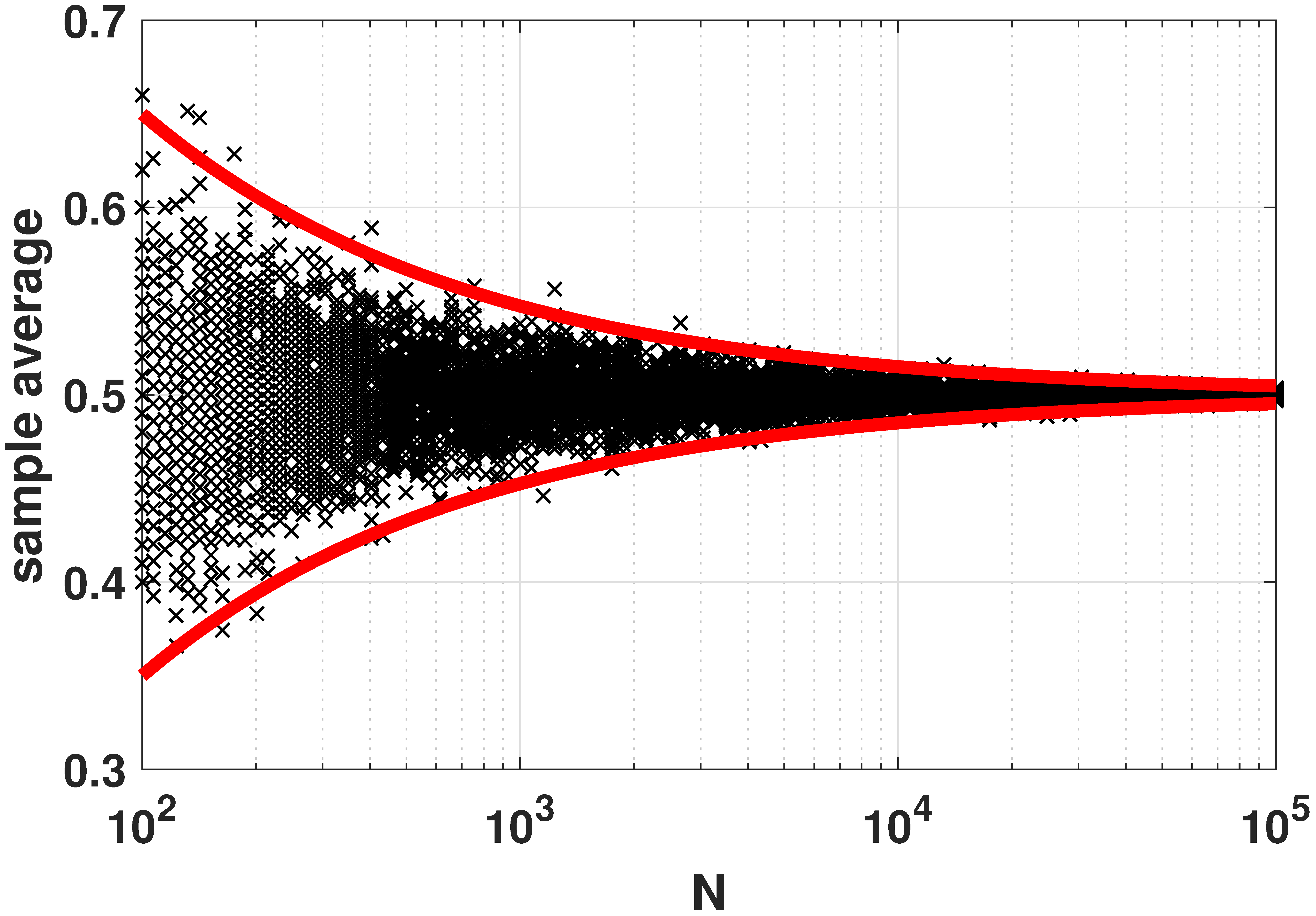
% MATLAB code to illustrate the weak law of large numbers
Nset = round(logspace(2,5,100));
for i=1:length(Nset)
    N = Nset(i);
    p = 0.5;
    x(:,i) = binornd(N, p, 1000,1)/N;
end
y = x(1:10:end,:)';
semilogx(Nset, y, 'kx'); hold on;
semilogx(Nset, p+3*sqrt(p*(1-p)./Nset), 'r', 'LineWidth', 4);
semilogx(Nset, p-3*sqrt(p*(1-p)./Nset), 'r', 'LineWidth', 4);

# Python code to illustrate the weak law of large numbers
import numpy as np
import matplotlib.pyplot as plt
import scipy.stats as stats
import numpy.matlib
p = 0.5
Nset = np.round(np.logspace(2,5,100)).astype(int)
x = np.zeros((1000,Nset.size))
for i in range(Nset.size):
  N = Nset[i]
  x[:,i] = stats.binom.rvs(N, p, size=1000)/N
Nset_grid = np.matlib.repmat(Nset, 1000, 1)
plt.semilogx(Nset_grid, x,'ko');
plt.semilogx(Nset, p + 3*np.sqrt((p*(1-p))/Nset), 'r', linewidth=6)
plt.semilogx(Nset, p - 3*np.sqrt((p*(1-p))/Nset), 'r', linewidth=6)

# Julia code to illustrate the weak law of large numbers
using Distributions, Plots

p = 0.5
Nset = round.((10).^range(2,5,length=100))
x = zeros(length(Nset), 1000)
for (i,N) in enumerate(Nset)
    x[i,:] = rand(Binomial(N, p), 1000) / N
end
y = x[:, 1:10:end]
scatter(Nset, y; xaxis=:log10, xticks=[1e2, 1e3, 1e4, 1e5],
        markershape=:x, color=:black,
        ylabel="sample average",
        legend=false)
plot!(Nset, p .+ 3*sqrt.(p*(1-p) ./ Nset); color=:red, linewidth=4)
plot!(Nset, p .- 3*sqrt.(p*(1-p) ./ Nset); color=:red, linewidth=4)

# R code to illustrate the weak law of large numbers

library(pracma)

p <- 0.5
Nset <- as.integer(round(logspace(2,5,100)))
x <- matrix(rep(0, 1000*length(Nset)), nrow=1000)
for (i in 1:length(Nset)) {
  N = Nset[i]
  x[,i] <- rbinom(1000, N, p) / N
}
Nset_grid <- repmat(Nset, m=1, n=1000)

semilogx(Nset_grid, x, col='black', pch=19)
points(Nset, p + 3*(((p*(1-p))/Nset)^(1/2)), col='red', pch=19, lwd=1)
points(Nset, p - 3*(((p*(1-p))/Nset)^(1/2)), col='red', pch=19, lwd=1)

% MATLAB: Plot the PDF of the sum of two Gaussians
figure;
n = 10000;
K = 2;
Z = zeros(1,n);
for i=1:K
    X = randi(6,1,n);
    Z = Z + X;
end
m = 3.5*K;
v = sqrt(K*(6^2-1)/12);
histogram(Z,K-0.5:6*K+0.5,'Normalization',...
    'probability','FaceColor',[0 0.5 0.8],'LineWidth',2);
set(gcf, 'Position', [100, 100, 600, 400]);
set(gca,'FontWeight','bold','fontsize',14);

# Python code to plot the PDF of the sum of two dice
import numpy as np
import matplotlib.pyplot as plt
n, K = 10000, 2
Z = np.zeros(n)
for i in range(K):
    Z = Z + np.random.randint(1, 7, size=n)
bins = np.arange(K - 0.5, 6*K + 1.5, 1)
plt.hist(Z, bins=bins, density=True, color=(0, 0.5, 0.8), edgecolor='k', linewidth=2)
plt.show()

# Julia: Plot the PDF of the sum of two Gaussians
using Distributions, Plots

n = 10000;
K = 2 # 6
X = DiscreteUniform(1, 6)
mu = mean(X)   # 3.5
sigma = std(X)    # sqrt((6^2-1)/12)
Z = sum(rand(X, n) for _ in 1:K)
mk = K * mu
sk = sqrt(K) * sigma
bin_range = (floor(mk - 3sk) - 1/2):(ceil(mk + 3sk) + 1/2)
plot_args = (normalize=true, color=RGB(0, 0.5, 0.8), linewidth=2, legend=false,
             bins=bin_range)

histogram(Z; plot_args..., title="⚁"^K)

# R: Plot the PDF of the sum of two Gaussians

library(pracma)

n <- 10000
K <- 2
Z <- rep(0, n)

for (i in 1:K) {
  X <- runif(n, min=1, max=6)
  Z <- Z + X
}
hist(Z,breaks=(K-0.5):(6*K+0.5),freq=FALSE)

% MATLAB: Visualize convergence in distribution
N = 10; % N = 50;
x = linspace(0,N,1001);
p = 0.5;
p_b = binopdf(x, N, p);
p_n = normpdf(x, N*p, sqrt(N*p*(1-p)));

c_b = binocdf(x, N, p);
c_n = normcdf(x, N*p, sqrt(N*p*(1-p)));

figure;
plot(x,p_b,'LineWidth',2,'Color',[0,0,0]); hold on;
plot(x,p_n,'LineWidth',6,'Color',[0.8,0,0]); hold off;
legend('Binomial', 'Gaussian', 'Location', 'Best');
grid on;
set(gcf, 'Position', [100, 100, 600, 400]);
set(gca,'FontWeight','bold','fontsize',14);

# Python code to visualize convergence in distribution
import numpy as np
import matplotlib.pyplot as plt
from scipy.stats import binom, norm
N, p = 10, 0.5            # try N = 50
k  = np.arange(0, N + 1)
xx = np.linspace(0, N, 1001)
fig, (ax1, ax2) = plt.subplots(1, 2)
ax1.stem(k, binom.pmf(k, N, p), linefmt='k-', markerfmt='ko', basefmt=' ')
ax1.plot(xx, norm.pdf(xx, N*p, np.sqrt(N*p*(1 - p))), color=(0.8, 0, 0), linewidth=4)
ax1.legend(['Binomial', 'Gaussian'])
ax2.step(k, binom.cdf(k, N, p), where='post', color='k')
ax2.plot(xx, norm.cdf(xx, N*p, np.sqrt(N*p*(1 - p))), color=(0.8, 0, 0), linewidth=4)
plt.show()

# Julia: Visualize convergence in distribution
using Distributions, Plots
N, p = 10, 0.5

B = Binomial(N,p)
Z = Normal(mean(B), std(B)) # N*p, sqrt(N*p*(1-p))

p_b(x) = pdf(B, x)
p_n(x) = pdf(Z, x)

c_b(x) = cdf(B, x)
c_n(x) = cdf(Z, x)

bin_args = (color = RGB(0, 0, 0), linewidth=2, label="Binomial")
norm_args = (color = RGB(0.8, 0, 0), linewidth=6, label="Normal")

ns = 0:N
p1 = plot(ns, p_b.(ns); bin_args..., seriestype=:sticks)
plot!(p_n, 0, N; norm_args...)

p2 = plot(c_b, 0, N; bin_args...)
plot!(c_n; norm_args...)

l = @layout [a b]
plot(p1, p2, layout=l)

# R: Visualize convergence in distribution

library(pracma)

N <- 10
N <- 50
x <- linspace(0, N, 1001)
p <- 0.5
p_b <- dbinom(x, N, p)
p_n <- dnorm(x, N*p, (N*p*(1-p))**(1/2))

c_b <- pbinom(x, N, p)
c_n <- pnorm(x, N*p, (N*p*(1-p))**(1/2))

plot(x, p_n, lwd=1, col='red')
lines(x, p_b, lwd=2, col='black')
legend("topright", c('Binomial', 'Gaussian'), fill=c('black', 'red'))

% MATLAB: Poisson to Gaussian: convergence in distribution
N = 4; % N = 10; % N = 50;
x = linspace(0,2*N,1001);
lambda = 1;
p_b = poisspdf(x, N*lambda);
p_n = normpdf(x, N*lambda, sqrt(N*lambda));

c_b = poisscdf(x, N*lambda);
c_n = normcdf(x, N*lambda, sqrt(N*lambda));

figure;
plot(x,p_b,'LineWidth',2,'Color',[0,0,0]); hold on;
plot(x,p_n,'LineWidth',6,'Color',[0.8,0,0]); hold off;
legend('Poisson', 'Gaussian', 'Location', 'NE');
grid on;
set(gcf, 'Position', [100, 100, 600, 400]);
set(gca,'FontWeight','bold','fontsize',18);

figure;
plot(x,c_b,'LineWidth',2,'Color',[0,0,0]); hold on;
plot(x,c_n,'LineWidth',6,'Color',[0.8,0,0]); hold off;
legend('Poisson', 'Gaussian', 'Location', 'SE');
grid on;
set(gcf, 'Position', [100, 100, 600, 400]);
set(gca,'FontWeight','bold','fontsize',18);

# Python code: Poisson to Gaussian convergence in distribution
import numpy as np
import matplotlib.pyplot as plt
from scipy.stats import poisson, norm
N, lam = 4, 1            # try N = 10, N = 50
k  = np.arange(0, 2*N + 1)
xx = np.linspace(0, 2*N, 1001)
fig, (ax1, ax2) = plt.subplots(1, 2)
ax1.stem(k, poisson.pmf(k, N*lam), linefmt='k-', markerfmt='ko', basefmt=' ')
ax1.plot(xx, norm.pdf(xx, N*lam, np.sqrt(N*lam)), color=(0.8, 0, 0), linewidth=4)
ax1.legend(['Poisson', 'Gaussian'])
ax2.step(k, poisson.cdf(k, N*lam), where='post', color='k')
ax2.plot(xx, norm.cdf(xx, N*lam, np.sqrt(N*lam)), color=(0.8, 0, 0), linewidth=4)
ax2.legend(['Poisson', 'Gaussian'])
plt.show()

# Julia: Poisson to Gaussian: convergence in distribution
using Distributions, Plots

N = 4; # N = 10, N = 50;
lambda = 1

P = Poisson(N*lambda)
Z = Normal(mean(P), std(P))  # Nlambda, sqrt(Nlambda)

p_b(x) = pdf(P, x) # evaluate on integers
p_n(x) = pdf(Z, x)

c_b(x) = cdf(P, x)
c_n(x) = cdf(Z, x)

bin_args = (linewidth=2, color=RGB(0.0, 0.0, 0.0), label="Poisson")
norm_args = (linewidth=6, color=RGB(0.8, 0.0, 0.0), label="Gaussian")

ns = 0:2N
p1 = plot(ns, p_b.(ns); bin_args..., seriestype=:sticks, legend=:topright)
plot!(p_n, 0, 2N; norm_args...)

p2 = plot(c_b, 0, 2N; bin_args..., legend=:bottomright)
plot!(c_n; norm_args...)

l = @layout [a b]
plot(p1, p2, layout=l)

# R: Poisson to Gaussian: convergence in distribution

library(pracma)

N <- 4
# N = 10
# N = 50

x <- linspace(0,2*N,1001)
lambda <- 1
p_b <- dpois(x, N*lambda)
p_n <- dnorm(x, N*lambda, sqrt(N*lambda))

c_b <- ppois(x, N*lambda);
c_n = pnorm(x, N*lambda, sqrt(N*lambda));

plot(x, p_n, col="red")
lines(x, p_b, col="black")
legend("topright", c('Poisson', 'Gaussian'), fill=c('black', 'red'))

plot(x, c_n, col="red")
lines(x, c_b, col="black")
legend("topright", c('Poisson', 'Gaussian'), fill=c('black', 'red'))

% MATLAB: Visualize the Central Limit Theorem
N = 10;
x = linspace(0,N,1001);
p = 0.5;
p_b = binopdf(x, N, p);
p_n = normpdf(x, N*p, sqrt(N*p*(1-p)));

c_b = binocdf(x, N, p);
c_n = normcdf(x, N*p, sqrt(N*p*(1-p)));

x2 = linspace(5-2.5,5+2.5,1001);
q2 = normpdf(x2,N*p, sqrt(N*p*(1-p)));

figure;
area(x2,q2,'EdgeColor','none','FaceColor',[0.6,0.9,1]); hold on;
plot(x,p_b,'LineWidth',2,'Color',[0,0,0]); 
grid on;
set(gcf, 'Position', [100, 100, 600, 400]);
set(gca,'FontWeight','bold','fontsize',14);

figure;
area(x2,q2,'EdgeColor','none','FaceColor',[0.6,0.9,1]); hold on;
plot(x,p_n,'LineWidth',6,'Color',[0.8,0,0]); 
grid on;
set(gcf, 'Position', [100, 100, 600, 400]);
set(gca,'FontWeight','bold','fontsize',14);

# Python code to visualize the Central Limit Theorem
import numpy as np
import matplotlib.pyplot as plt
from scipy.stats import binom, norm
N, p = 10, 0.5
k  = np.arange(0, N + 1)
xx = np.linspace(0, N, 1001)
x2 = np.linspace(5 - 2.5, 5 + 2.5, 1001)
q2 = norm.pdf(x2, N*p, np.sqrt(N*p*(1 - p)))
plt.figure()
plt.fill_between(x2, q2, color=(0.6, 0.9, 1))
plt.stem(k, binom.pmf(k, N, p), linefmt='k-', markerfmt='ko', basefmt=' ')
plt.grid(True)
plt.figure()
plt.fill_between(x2, q2, color=(0.6, 0.9, 1))
plt.plot(xx, norm.pdf(xx, N*p, np.sqrt(N*p*(1 - p))), color=(0.8, 0, 0), linewidth=6)
plt.grid(True); plt.show()

# Julia: Visualize the Central Limit Theorem
using Distributions, Plots

N = 10
x = range(0, N, length=1001)
p = 0.5


B = Binomial(N,p)
Z = Normal(mean(B), std(B))  # N*p, sqrt(N*p*(1-p))

p_b(x) = pdf(B, x)
p_n(x) = pdf(Z, x)

c_b(x) = cdf(B, x)
c_n(x) = cdf(Z, x)


xs = range(5-2.5, 5 + 2.5, length=1001)

p1 = plot(p_n, 5-2.5, 5+2.5; fillrange=0 .* xs, color=RGB(0.6, 0.9, 1.0), legend=false,
     title="Binomial PDF")
plot!(0:N, p_b.(0:N); color=RGB(0,0,0), linewidth=2, seriestype=:sticks, layout=1)


p2 = plot(p_n, 5-2.5, 5+2.5, fillrange=0 .* xs, color=RGB(0.6, 0.9, 1.0), legend=false,
     title = "Gaussian PDF")
plot!(p_n, 0, N; color=RGB(0.8, 0, 0), linewidth=6, layout=2)

l = @layout [a b]
plot(p1, p2, layout=l)

# R: Visualize the Central Limit Theorem

library(pracma)

N <- 10
x <- linspace(0,N,1001)
p <- 0.5
p_b <- dbinom(x, N, p);
p_n <- dnorm(x, N*p, sqrt(N*p*(1-p)));

c_b <- pbinom(x, N, p);
c_n <- pnorm(x, N*p, sqrt(N*p*(1-p)));

x2 <- linspace(5-2.5,5+2.5,1001);
q2 <- dnorm(x2,N*p, sqrt(N*p*(1-p)));

plot(x, p_n, col="red")
points(x, p_b, col="black", pch=19)

polygon(c(min(x2), x2, max(x2)), c(0, q2, 0), col='lightblue')

% MATLAB: Central Limit Theorem from moment generating functions
p = 0.5;
s = linspace(-10,10,1001);
MX = 1-p+p*exp(s);
N = 2;  
semilogy(s, (1-p+p*exp(s/N)).^N, 'LineWidth',8, 'Color',[0.1,0.6,1]); hold on;
mu = p;
sigma = sqrt(p*(1-p)/N);
MZ = exp(mu*s + sigma^2*s.^2/2);
semilogy(s, MZ,':','LineWidth', 8, 'Color',[0,0,0]);
grid on;
axis([-10, 10 1e-2 1e5]);
legend('Binomial MGF', 'Gaussian MGF','Location','NW');
yticks([1e-2 1e-1 1 1e1 1e2 1e3 1e4 1e5]);
set(gcf, 'Position', [100, 100, 600, 400]);
set(gca,'FontWeight','bold','fontsize',24);

# Python code: Central Limit Theorem from moment generating functions
import numpy as np
import matplotlib.pyplot as plt
p = 0.5
s = np.linspace(-10, 10, 1001)
N = 2
M_binom = (1 - p + p*np.exp(s/N))**N
mu, sigma = p, np.sqrt(p*(1 - p)/N)
M_gauss = np.exp(mu*s + sigma**2*s**2/2)
plt.semilogy(s, M_binom, linewidth=8, color=(0.1, 0.6, 1), label='Binomial MGF')
plt.semilogy(s, M_gauss, ':', linewidth=8, color='k', label='Gaussian MGF')
plt.axis([-10, 10, 1e-2, 1e5]); plt.legend(); plt.grid(True); plt.show()

# Julia: Central Limit Theorem from moment generating functions
using Distributions, Plots

N = 2
p = 0.5;

B = Bernoulli(p)
mu, sigma = mean(B), std(B)/sqrt(N) # for Xbar
Z = Normal(mu, sigma)

m_Bernoulli(s) = mgf(B,s)    # (1 - p + p*exp(s))
m_B(s) = m_Bernoulli(s/N)^N  # (X1 + X2 + ... XN)/N
m_Z(s) = mgf(Z,s)            # exp(mu * s + sigma^2*s^2/2)

bin_args = (linewidth=8, color=RGB(0.1, 0.6, 1),
            yaxis=:log, yticks = [10.0^i for i in -1:4],
            label="Binomial MGF")
norm_args = (linewidth=8, color=RGB(0, 0, 0), yaxis=:log, linestyle=:dot, label="Gaussian MGF")

plot(m_B, -10, 10; bin_args..., legend=:topleft)
plot!(m_Z; norm_args...)

# R: How moment generating of Gaussian approximates in CLT

library(pracma)

p <- 0.5
s <- linspace(-10,10,1001)
MX <- 1-p+p*exp(s)
N <- 2
semilogy(s, (1-p+p*exp(s/N))**N, lwd=4, col="lightblue", xlim=c(-10,10), ylim=c(10**-2, 10**5))
mu <- p
sigma <- sqrt(p*(1-p)/N);
MZ <- exp(mu*s + sigma^2*s**2/2);
lines(s, MZ, lwd=4);
legend("topleft", c('Binomial MGF', 'Gaussian MGF'), fill=c('lightblue', 'black'))

% MATLAB: Failure of Central Limit Theorem at tails
x = linspace(-1,5,1001);
lambda = 1;

N = 1;
f1 = (sqrt(N)/lambda)*pdf('gamma',(x+sqrt(N))/(lambda/sqrt(N)),N,lambda);
semilogy(x, f1, 'LineWidth', 4, 'Color', [0.8 0.8 0.8]); hold on;

N = 10;
f2 = (sqrt(N)/lambda)*pdf('gamma',(x+sqrt(N))/(lambda/sqrt(N)),N,lambda);
semilogy(x, f2, 'LineWidth', 4, 'Color', [0.6 0.6 0.6]); 

N = 100;
f3 = (sqrt(N)/lambda)*pdf('gamma',(x+sqrt(N))/(lambda/sqrt(N)),N,lambda);
semilogy(x, f3, 'LineWidth', 4, 'Color', [0.4 0.4 0.4]); 

N = 1000;
f4 = (sqrt(N)/lambda)*pdf('gamma',(x+sqrt(N))/(lambda/sqrt(N)),N,lambda);
semilogy(x, f4, 'LineWidth', 4, 'Color', [0.2 0.2 0.2]); 

g = pdf('norm',x,0,1);
semilogy(x, g, '-.', 'LineWidth', 4, 'Color', [0.9 0.0 0.0]);

grid on;
legend('N = 1', 'N = 10', 'N = 100', 'N = 1000', 'Gaussian', 'Location','SW');
axis([-1 5 min(ylim) max(ylim)]);
set(gcf, 'Position', [100, 100, 600, 400]);
set(gca,'FontWeight','bold','fontsize',18);

# Python code: Failure of the Central Limit Theorem at the tails
import numpy as np
import matplotlib.pyplot as plt
from scipy.stats import gamma, norm
x = np.linspace(-1, 5, 1001)
lam = 1
def shifted_gamma(N):
    return (np.sqrt(N)/lam)*gamma.pdf((x + np.sqrt(N))/(lam/np.sqrt(N)), N, scale=lam)
shades = {1: (0.8,)*3, 10: (0.6,)*3, 100: (0.4,)*3, 1000: (0.2,)*3}
for N, c in shades.items():
    plt.semilogy(x, shifted_gamma(N), linewidth=4, color=c, label=f'N = {N}')
plt.semilogy(x, norm.pdf(x, 0, 1), '-.', linewidth=4, color=(0.9, 0, 0), label='Gaussian')
plt.legend(); plt.grid(True); plt.show()

# Julia: Failure of Central Limit Theorem at tails
using Distributions, Plots


lambda = 1;

function gamma_pdf(N)
    function(x) # return anonymous function; also x -> ... notation
        (sqrt(N)/lambda) * pdf(Gamma(N,lambda), (x+sqrt(N))/(lambda/sqrt(N)))
    end
end
gaussian_pdf(x) = pdf(Normal(), x)


plot(gamma_pdf(1), -1, 5; linewidth=4, color=RGB(0.8, 0.8, 0.8), label="N=1",
     yaxis=:log,
     legend=:bottomleft)
plot!(gamma_pdf(10);   linewidth=4, color=RGB(0.6, 0.6, 0.6), label="N=10")
plot!(gamma_pdf(100);  linewidth=4, color=RGB(0.4, 0.4, 0.4), label="N=100")
plot!(gamma_pdf(1000); linewidth=4, color=RGB(0.2, 0.2, 0.2), label="N=1000")
plot!(gaussian_pdf;    linewidth=4, color=RGB(0.9, 0.0, 0.0), label="Gaussian",
      linestyle=:dash)

# R: Failure of Central Limit Theorem at tails

library(pracma)

x <- linspace(-1,5,1001)
lambda <- 1

N <- 1
f1 <- (N**(1/2)/lambda)*dgamma((x+sqrt(N))/(lambda/sqrt(N)), N, lambda)
semilogy(x, f1, lwd=1, col='lightgray', xlim=c(-1,5), ylim=c(10**-6, 1))

N <- 10
f1 <- (N**(1/2)/lambda)*dgamma((x+sqrt(N))/(lambda/sqrt(N)), N, lambda)
lines(x, f1, lwd=2, col='gray')

N <- 100
f1 <- (N**(1/2)/lambda)*dgamma((x+sqrt(N))/(lambda/sqrt(N)), N, lambda)
lines(x, f1, lwd=2, col='darkgray')

N <- 1000
f1 <- (N**(1/2)/lambda)*dgamma((x+sqrt(N))/(lambda/sqrt(N)), N, lambda)
lines(x, f1, lwd=2, col='black')

g <- dnorm(x,0,1)
lines(x, g, lwd=2, pch=1, col='red')

legend("bottomleft", c('N=1', 'N=10', 'N=100', 'N=1000', 'Gaussian'), fill=c('lightgray', 'gray', 'darkgray', 'black', 'red'))

# MATLAB code to fit data points using a straight line
N = 50;
x = rand(N,1)*1;
a = 2.5;                         % true parameter
b = 1.3;                         % true parameter
y = a*x + b + 0.2*rand(size(x)); % Synthesize training data

X    = [x(:) ones(N,1)];         % construct the X matrix
theta = X\y(:);                  % solve y = X theta

t    = linspace(0, 1, 200);      % interpolate and plot
yhat = theta(1)*t + theta(2);
plot(x,y,'o','LineWidth',2); hold on;
plot(t,yhat,'r','LineWidth',4);

# Python code to fit data points using a straight line
import numpy as np
import matplotlib.pyplot as plt

N = 50
x = np.random.rand(N)
a = 2.5                                 # true parameter
b = 1.3                                 # true parameter
y = a*x + b + 0.2*np.random.randn(N)    # Synthesize training data

X = np.column_stack((x, np.ones(N)))    # construct the X matrix
theta = np.linalg.lstsq(X, y, rcond=None)[0] # solve y = X theta

t = np.linspace(0,1,200)                # interpolate and plot
yhat = theta[0]*t + theta[1]
plt.plot(x,y,'o')
plt.plot(t,yhat,'r',linewidth=4)

# Julia code to fit data points using a straight line
N = 50
x = rand(N)
a = 2.5                         # true parameter
b = 1.3                         # true parameter
y = a*x .+ b + 0.2*rand(N)      # Synthesize training data

X = [x ones(N)]                 # construct the X matrix
theta = X\y                         # solve y = X*theta

t    = range(0,stop=1,length=200)
yhat = theta[1]*t .+ theta[2]                  # fitted values at t

p1 = scatter(x,y,markershape=:circle,label="data",legend=:topleft)
plot!(t,yhat,linecolor=:red,linewidth=4,label="best fit")
display(p1)

# R code to fit data points using a straight line

library(pracma)

N <- 50
x <- runif(N)

a <- 2.5 # true parameter
b <- 1.3 # true parameter
y <- a*x + b + 0.2*rnorm(N) # Synthesize training data

X <- cbind(x, rep(1, N))
theta <- lsfit(X, y)$coefficients
t <- linspace(0, 1, 200)
yhat <- theta[2]*t + theta[1]
plot(x, y, pch=19)
lines(t, yhat, col='red', lwd=4)
legend("bottomright", c("Best Fit", "Data"), fill=c("red", "black"))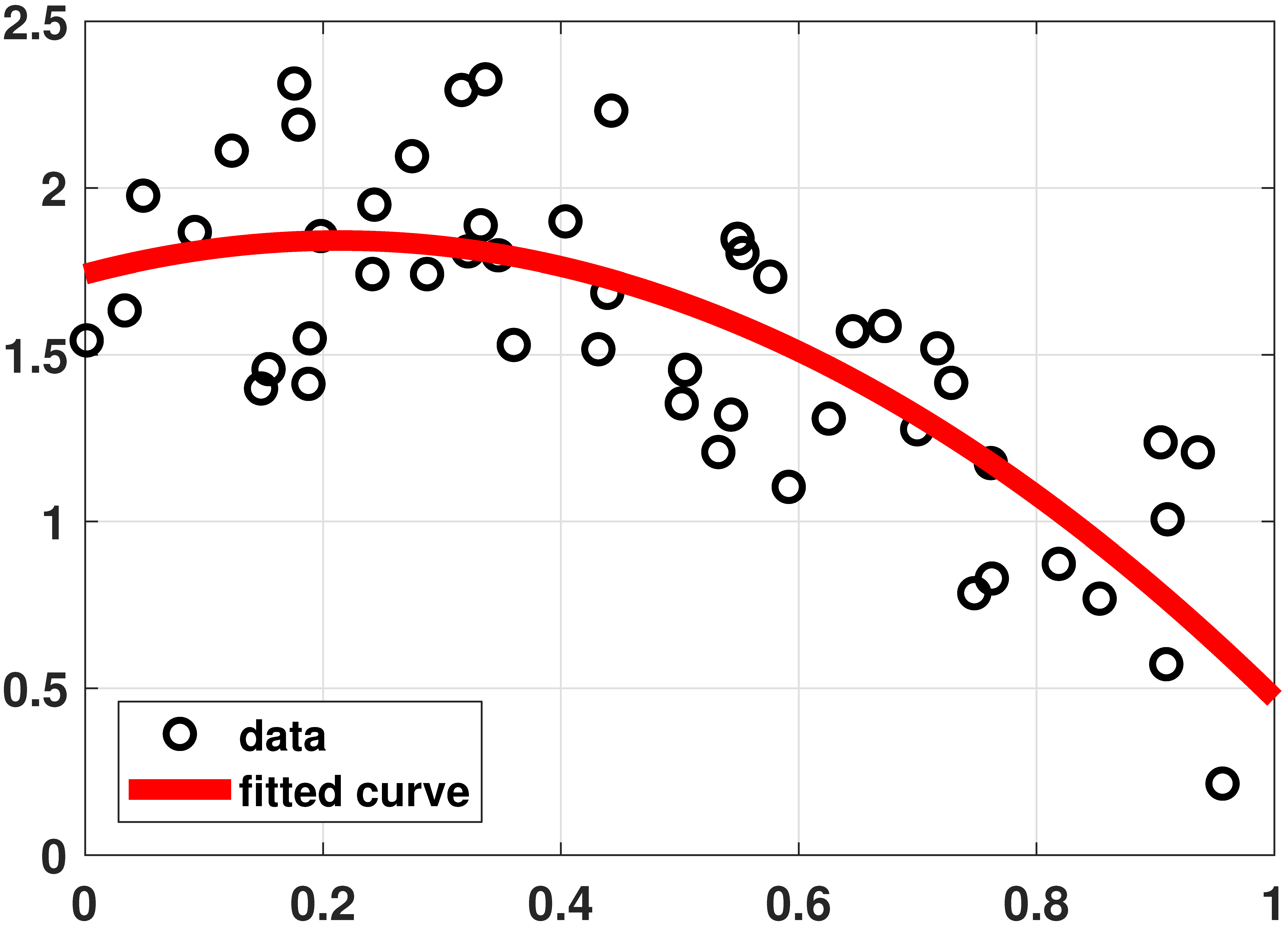

% MATLAB code to fit data using a quadratic equation
N = 50;
x = rand(N,1)*1;
a = -2.5;
b = 1.3;
c = 1.2;
y = a*x.^2 + b*x + c + 1*rand(size(x));

N    = length(x);
X    = [ones(N,1) x(:) x(:).^2];
beta = X\y(:);
t    = linspace(0, 1, 200);
yhat = theta(3)*t.^2 + theta(2)*t + theta(1);
plot(x,y,   'o','LineWidth',2); hold on;
plot(t,yhat,'r','LineWidth',6);

# Python code to fit data using a quadratic equation
import numpy as np
import matplotlib.pyplot as plt

N = 50
x = np.random.rand(N)
a = -2.5
b = 1.3
c = 1.2
y = a*x**2 + b*x + c + 0.2*np.random.randn(N)

X = np.column_stack((np.ones(N), x, x**2))
theta = np.linalg.lstsq(X, y, rcond=None)[0]
t = np.linspace(0,1,200)
yhat = theta[0] + theta[1]*t + theta[2]*t**2
plt.plot(x,y,'o')
plt.plot(t,yhat,'r',linewidth=4)

# Julia code to fit data using a quadratic equation
N = 50
x = rand(N)
a = -2.5
b = 1.3
c = 1.2
X = x.^[0 1 2]                #same as [ones(N) x x.^2]
y = X*[c,b,a] + rand(N)

theta    = X\y
t    = range(0,stop=1,length=200)
yhat = (t.^[0 1 2])*theta               #same as (t.^collect(0:2)')*theta

p2 = scatter(x,y,markershape=:circle,label="data",legend=:bottomleft)
plot!(t,yhat,linecolor=:red,linewidth=4,label="fitted curve")
display(p2)

# R code to fit data using a quadratic equation

N <- 50
x <- runif(N)
a <- -2.5
b <- 1.3
c <- 1.2
y <- a*x**2 + b*x + c + 0.2*rnorm(N)
X <- cbind(rep(1, N), x, x**2)
theta <- lsfit(X, y)$coefficients
t = linspace(0, 1, 200)
print(theta)
yhat = theta[1] + theta[2]*t + theta[3]*t**2
plot(x,y,pch=19)
lines(t,yhat,col='red',lwd=4)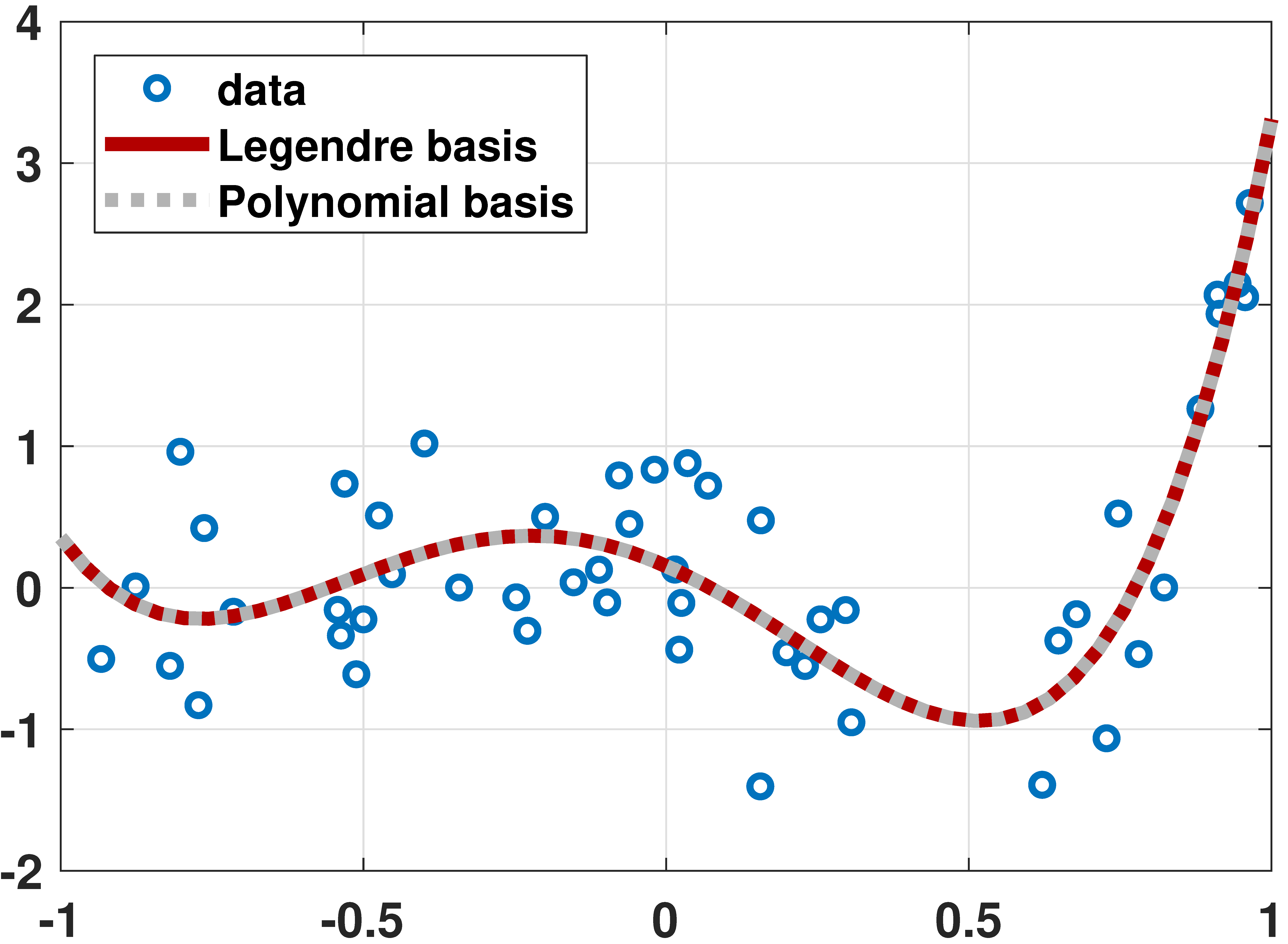

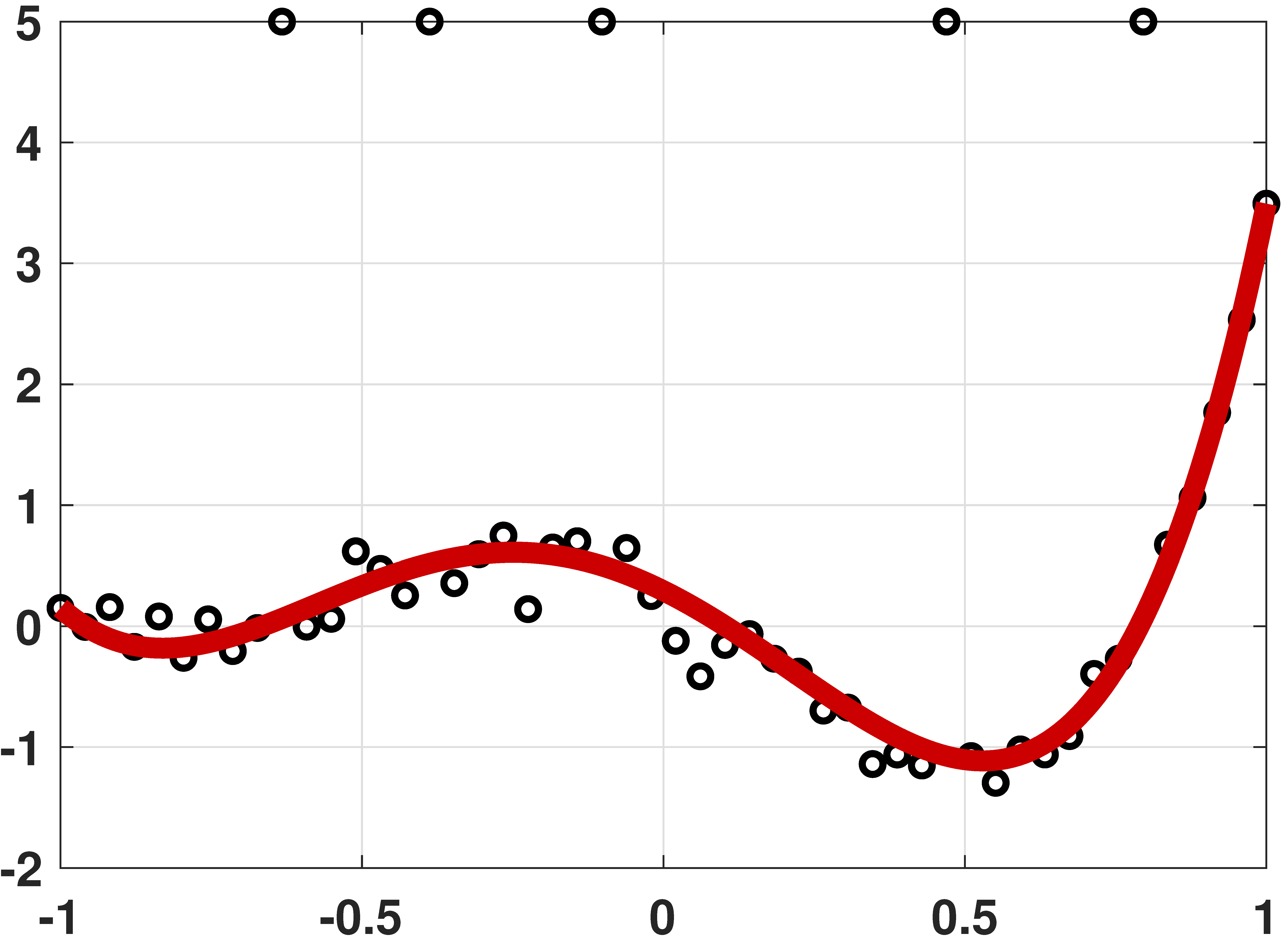
% MATLAB code to fit data using Legendre polynomials
N = 50;
x = 1*(rand(N,1)*2-1);
a = [-0.001 0.01 +0.55 1.5 1.2];
y = a(1)*legendreP(0,x) + a(2)*legendreP(1,x) + ...
  + a(3)*legendreP(2,x) + a(4)*legendreP(3,x) + ...
  + a(5)*legendreP(4,x) + 0.5*randn(N,1);

X = [legendreP(0,x(:)) legendreP(1,x(:)) ...
     legendreP(2,x(:)) legendreP(3,x(:)) ...
     legendreP(4,x(:))];
beta = X\y(:);

t    = linspace(-1, 1, 200);
yhat = beta(1)*legendreP(0,t) + beta(2)*legendreP(1,t) + ...
     + beta(3)*legendreP(2,t) + beta(4)*legendreP(3,t) + ...
     + beta(5)*legendreP(4,t);
plot(x,y,'ko','LineWidth',2,'MarkerSize',10); hold on;
plot(t,yhat,'LineWidth',6,'Color',[0.9 0 0]);

import numpy as np
import matplotlib.pyplot as plt
from scipy.special import eval_legendre

N = 50
x = np.linspace(-1,1,N)
a = np.array([-0.001, 0.01, 0.55, 1.5, 1.2])
y = a[0]*eval_legendre(0,x) + a[1]*eval_legendre(1,x) + \
    a[2]*eval_legendre(2,x) + a[3]*eval_legendre(3,x) + \
    a[4]*eval_legendre(4,x) + 0.2*np.random.randn(N)

X = np.column_stack((eval_legendre(0,x), eval_legendre(1,x), \
                     eval_legendre(2,x), eval_legendre(3,x), \
                     eval_legendre(4,x)))
theta = np.linalg.lstsq(X, y, rcond=None)[0]
t     = np.linspace(-1, 1, 50);
yhat  = theta[0]*eval_legendre(0,t) + theta[1]*eval_legendre(1,t) + \
        theta[2]*eval_legendre(2,t) + theta[3]*eval_legendre(3,t) + \
        theta[4]*eval_legendre(4,t)
plt.plot(x,y,'o',markersize=12)
plt.plot(t,yhat, linewidth=8)
plt.show()

# Julia code to fit data using Legendre polynomials

using LegendrePolynomials

N = 50
x = rand(N)*2 .- 1
a = [-0.001, 0.01, 0.55, 1.5, 1.2]
X = hcat([Pl.(x,p) for p=0:4]...)   # same as [Pl.(x,0) Pl.(x,1) Pl.(x,2) Pl.(x,3) Pl.(x,4)]
y = X*a + 0.5*randn(N)
theta = X\y

t    = range(-1,stop=1,length=200)
yhat = hcat([Pl.(t,p) for p=0:4]...)*theta

p3 = scatter(x,y,markershape=:circle,label="data",legend=:bottomleft)
plot!(t,yhat,linecolor=:red,linewidth=4,label="fitted curve")
display(p3)

# R code to fit data using Legendre polynomials

library(pracma)

N <- 50
x <- linspace(-1,1,N)
a <- c(-0.001, 0.01, 0.55, 1.5, 1.2)
y <- a[1]*legendre(0, x) + a[2]*legendre(1, x)[1,] + 
  a[3]*legendre(2, x)[1,] + a[4]*legendre(3, x)[1,] + 
  a[5]*legendre(4, x)[1,] + 0.2*rnorm(N)

X <- cbind(legendre(0, x), legendre(1, x)[1,], 
           legendre(2, x)[1,], legendre(3, x)[1,],
           legendre(4, x)[1,]) # good

beta <- mldivide(X, y)

t <- linspace(-1, 1, 50)
yhat <- beta[1]*legendre(0, x) + beta[2]*legendre(1, x)[1,] + 
  beta[3]*legendre(2, x)[1,] + beta[4]*legendre(3, x)[1,] + 
  beta[5]*legendre(4, x)[1,]

plot(x, y, pch=19, col="blue")
lines(t, yhat, lwd=2, col="orange")

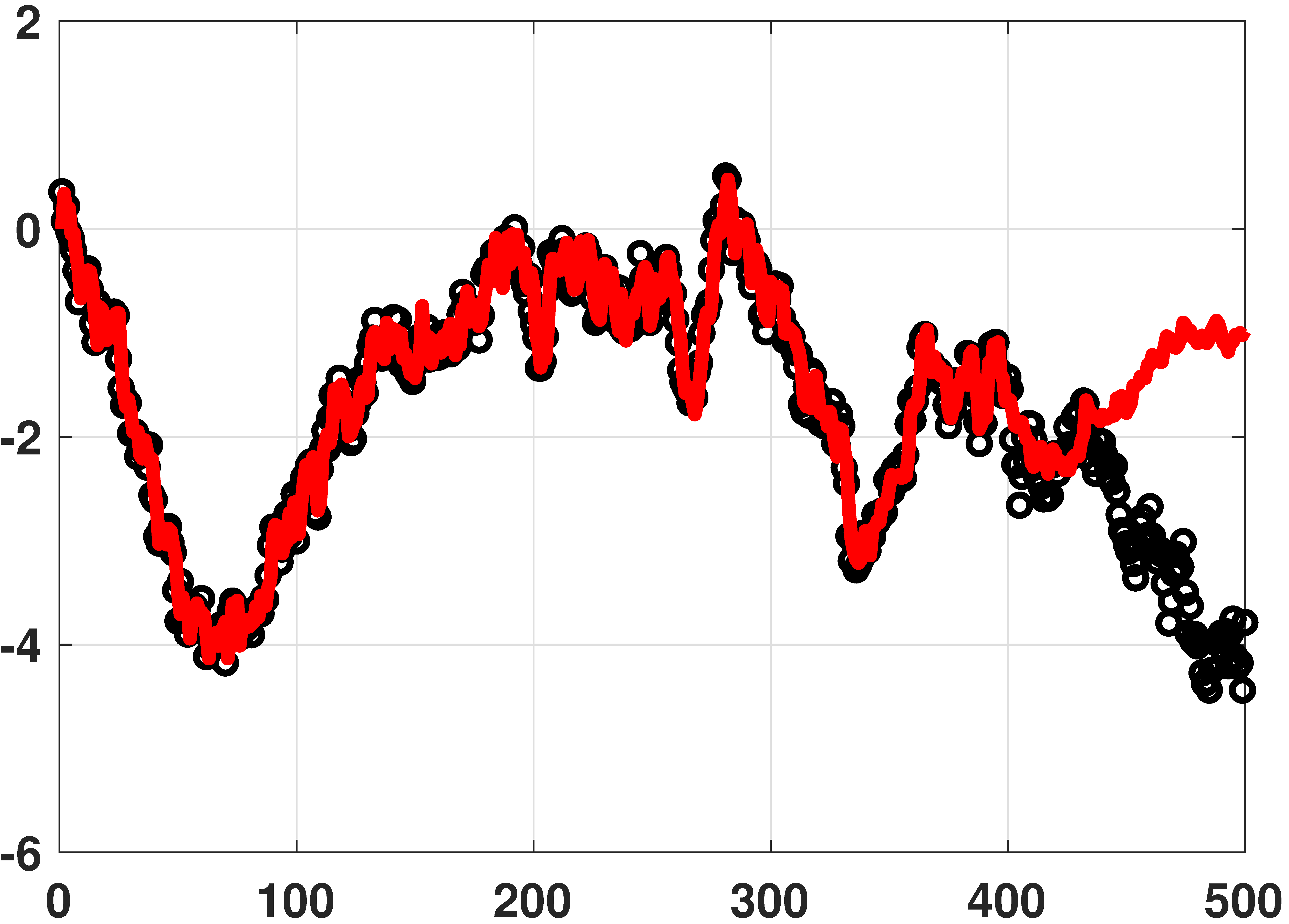
% MATLAB code for auto-regressive model
N = 500;
y = cumsum(0.2*randn(N,1)) + 0.05*randn(N,1);   % generate data

L = 100;                                        % use previous 100 samples
c = [0; y(1:400-1)];
r = zeros(1,L);
X = toeplitz(c,r);                              % Toeplitz matrix
theta = X\y(1:400);                             % solve y = X theta
yhat = X*theta;                                 % prediction
plot(y(1:400),   'ko','LineWidth',2);hold on;
plot(yhat(1:400),'r','LineWidth',4);

# Python code for auto-regressive model
import numpy as np
import matplotlib.pyplot as plt
from scipy.linalg import toeplitz

N = 500
y = np.cumsum(0.2*np.random.randn(N)) + 0.05*np.random.randn(N)

L = 100
c = np.hstack((0, y[0:400-1]))
r = np.zeros(L)
X = toeplitz(c,r)
theta = np.linalg.lstsq(X, y[0:400], rcond=None)[0]
yhat  = np.dot(X, theta)
plt.plot(y[0:400], 'o')
plt.plot(yhat[0:400],linewidth=4)

# Julia code for auto-regressive model
using ToeplitzMatrices

N = 500
y = cumsum(0.2*randn(N)) + 0.05*randn(N)        # generate data

L = 100                                         # use previous 100 samples
c = [0; y[1:400-1]]
r = zeros(L)
X = Matrix(Toeplitz(c,r))                       # Toeplitz matrix, converted
theta = X\y[1:400]                                  # solve y = X*theta
yhat = X*theta                                      # prediction

p4 = scatter(y[1:400],markershape=:circle,label="data",legend=:bottomleft)
plot!(yhat[1:400],linecolor=:red,linewidth=4,label="fitted curve")
display(p4)

# R code for auto-regressive model

library(pracma)

N <- 500
y <- cumsum(0.2*rnorm(N)) + 0.05*rnorm(N)

L <- 100
c <- c(0, y[0:(400-1)])
r = rep(0, L)
X = Toeplitz(c,r)
beta <- mldivide(X, y[1:400])
yhat  = X %*% beta
plot(y[1:400])
lines(yhat[1:400], col="red")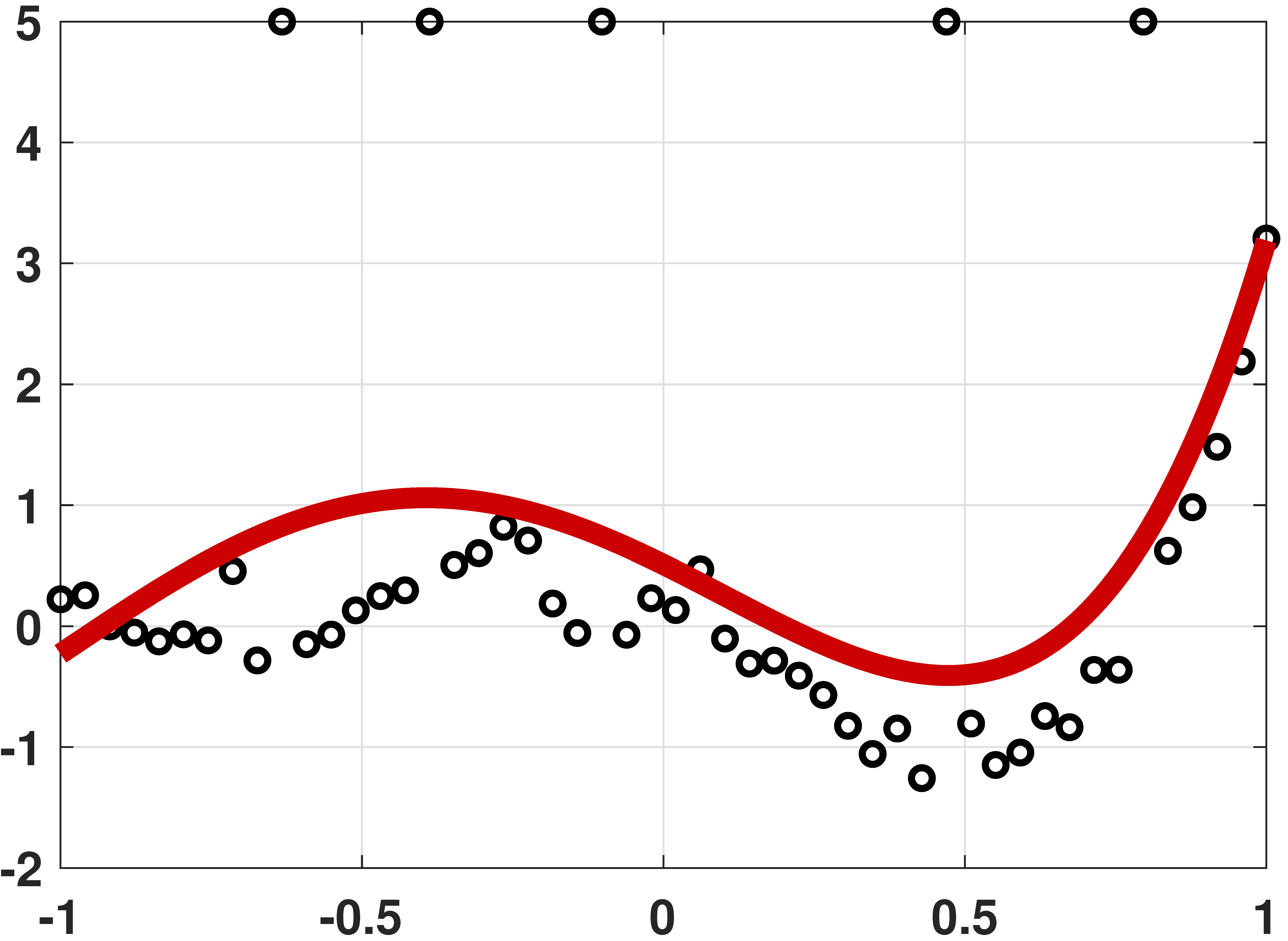

% MATLAB code to demonstrate robust regression
N = 50;
x = linspace(-1,1,N)';
a = [-0.001 0.01 0.55 1.5 1.2];
y = a(1)*legendreP(0,x) + a(2)*legendreP(1,x) + ...
    a(3)*legendreP(2,x) + a(4)*legendreP(3,x) + ...
    a(5)*legendreP(4,x) + 0.2*randn(N,1);
idx  = [10, 16, 23, 37, 45];
y(idx) = 5;

X    = [x(:).^0 x(:).^1 x(:).^2 x(:).^3 x(:).^4];
A    = [X -eye(N); -X -eye(N)];
b    = [y(:); -y(:)];
c    = [zeros(1,5) ones(1,N)]';
theta = linprog(c, A, b);

t    = linspace(-1,1,200)';
yhat = theta(1) + theta(2)*t(:) + ...
       theta(3)*t(:).^2 + theta(4)*t(:).^3 + ...
       theta(5)*t(:).^4;
plot(x,y,   'ko','LineWidth',2); hold on;
plot(t,yhat,'r','LineWidth',4);

# Python code to demonstrate robust regression
import numpy as np
import matplotlib.pyplot as plt
from scipy.special import eval_legendre
from scipy.optimize import linprog

N = 50
x = np.linspace(-1,1,N)
a = np.array([-0.001, 0.01, 0.55, 1.5, 1.2])
y = a[0]*eval_legendre(0,x) + a[1]*eval_legendre(1,x) + \
    a[2]*eval_legendre(2,x) + a[3]*eval_legendre(3,x) + \
    a[4]*eval_legendre(4,x) + 0.2*np.random.randn(N)
idx = [10,16,23,37,45]
y[idx] = 5
X = np.column_stack((np.ones(N), x, x**2, x**3, x**4))
A = np.vstack((np.hstack((X, -np.eye(N))), np.hstack((-X, -np.eye(N)))))
b = np.hstack((y,-y))
c = np.hstack((np.zeros(5), np.ones(N)))
res = linprog(c, A, b, bounds=(None,None), method="revised simplex")
theta = res.x
t    = np.linspace(-1,1,200)
yhat = theta[0]*np.ones(200) + theta[1]*t + theta[2]*t**2 + \
       theta[3]*t**3 + theta[4]*t**4
plt.plot(x,y,'o',markersize=12)
plt.plot(t,yhat, linewidth=8)
plt.show()

# Julia code to demonstrate robust regression

using LinearAlgebra, LegendrePolynomials, Convex, SCS
import MathOptInterface
const MOI = MathOptInterface

#----------------------------------------------------------
"""
    linprog_Convex(c,A,sense,b)
A wrapper for doing linear programming with Convex.jl/SCS.jl.
It solves, for instance, `c'x` st. `A*x<=b`
"""
function linprog_Convex(c,A,sense,b)
    n  = length(c)
    x  = Variable(n)
    #c1 = sense(A*x,b)             #restriction, for Ax <= b, use sense = (<=)
    c1 = A*x <= b
    prob = minimize(dot(c,x),c1)
    solve!(prob,()->SCS.Optimizer(verbose = false))
    x_i = prob.status == MOI.OPTIMAL ? vec(evaluate(x)) : NaN
    return x_i
end
#----------------------------------------------------------

N = 50
x = range(-1,stop=1,length=N)
a = [-0.001, 0.01, 0.55, 1.5, 1.2]
y = hcat([Pl.(x,p) for p=0:4]...)*a  + 0.05*randn(N)        # generate data
idx     = [10, 16, 23, 37, 45]
y[idx] .= 5

X = x.^[0 1 2 3 4]
A = [X -I; -X -I]
b = [y; -y]
c = [zeros(5);ones(N)]

theta = linprog_Convex(c,A,(<=),b)

t    = range(-1,stop=1,length=200)
yhat = (t.^[0 1 2 3 4])*theta[1:5]

p5 = scatter(x,y,markershape=:circle,label="data",legend=:bottomleft)
plot!(t,yhat,linecolor=:red,linewidth=4,label="fitted curve")
display(p5)

# R code to demonstrate robust regression
library(pracma)

N <- 50
x <- linspace(-1,1,N)
a <- c(-0.001, 0.01, 0.55, 1.5, 1.2)
y <- a[1]*legendre(0, x) + a[2]*legendre(1, x)[1,] + 
  a[3]*legendre(2, x)[1,] + a[4]*legendre(3, x)[1,] + 
  a[5]*legendre(4, x)[1,] + 0.2*rnorm(N)

idx <- c(10, 16, 23, 37, 45)
y[idx] <- 5

X <- cbind(rep(1,N), x, x**2, x**3, x**4)
A <- rbind(cbind(X, -1*diag(N)), cbind(-X, -1*diag(N)))
b <- c(y, -y)
c <- c(rep(0, 5), rep(1, N))
res <- linprog(c, A, b, maxiter=1000000)
beta <- res.x
t <- linspace(-1, 1, 200)

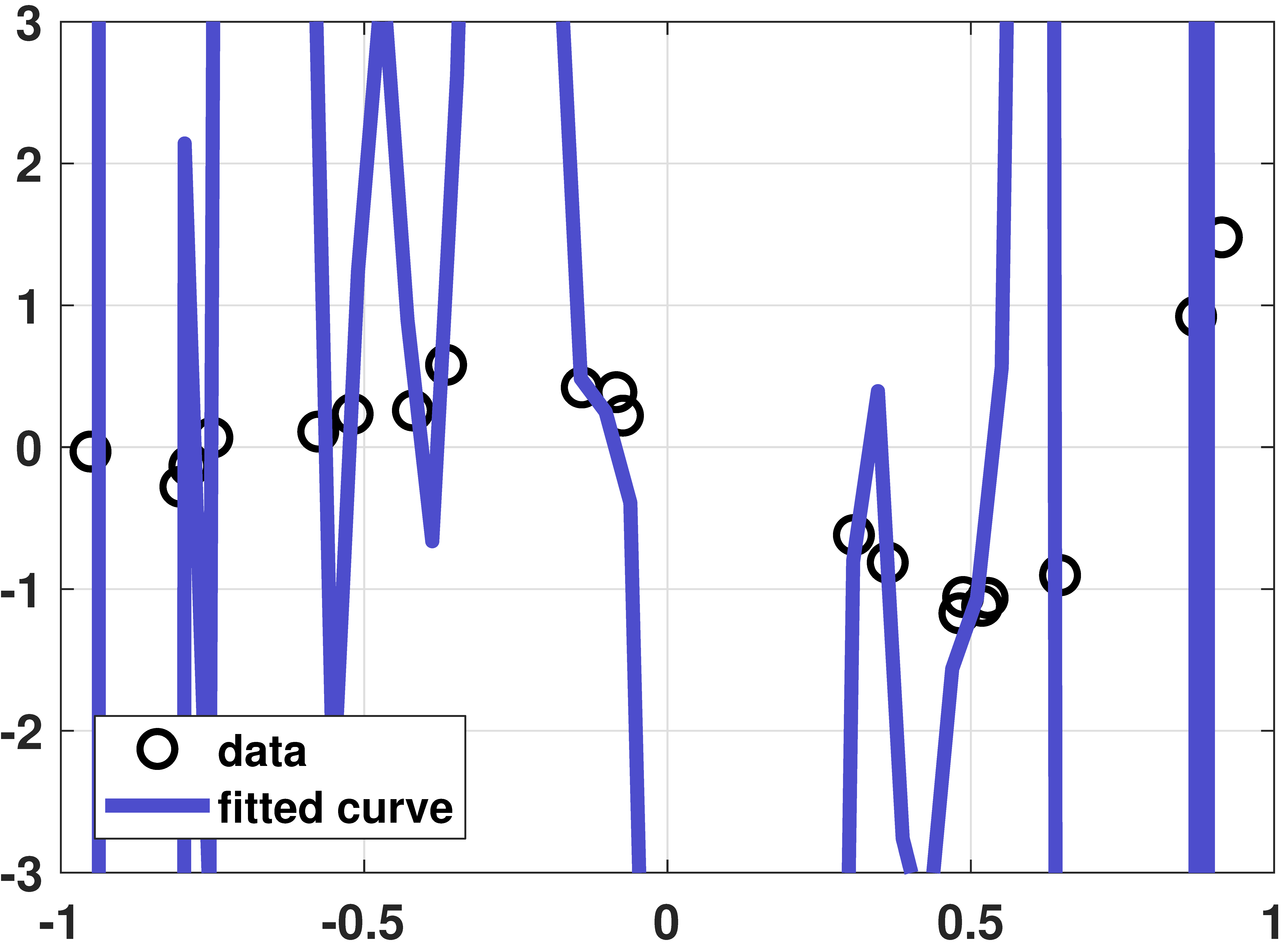
% MATLAB: An overfitting example
N = 20;
x = sort(1*(rand(N,1)*2-1));
a = [-0.001 0.01 +0.55 1.5 1.2];
y = a(1)*legendreP(0,x) + a(2)*legendreP(1,x) + ...
    a(3)*legendreP(2,x) + a(4)*legendreP(3,x) + ...
    a(5)*legendreP(4,x) + 0.1*randn(N,1);

figure(1);
P = 20;
X = zeros(N, P+1);
for p=0:P
    tmp = legendreP(p,x);
    X(:,p+1) = tmp(:);
end
beta = X\y;

t    = linspace(-1, 1, 50);
Xhat = zeros(length(t), P+1);
for p=0:P
    tmp = legendreP(p,t);
    Xhat(:,p+1) = tmp(:);
end
yhat = Xhat*beta;
plot(x,y,   'ko','LineWidth',2, 'MarkerSize', 10); hold on;
plot(t,yhat,'LineWidth',4,'Color',[0.3 0.3 0.8]);
legend('data', 'fitted curve','Location','SW');
grid on;
set(gcf, 'Position', [100, 100, 600, 400]);
set(gca,'FontWeight','bold','fontsize',14);
axis([-1 1 -3 3]);

# Python code: An overfitting example
import numpy as np
import matplotlib.pyplot as plt
from scipy.special import eval_legendre
N = 20
x = np.sort(np.random.rand(N)*2 - 1)
a = np.array([-0.001, 0.01, 0.55, 1.5, 1.2])
y = sum(a[p]*eval_legendre(p, x) for p in range(5)) + 0.1*np.random.randn(N)
P = 20
X = np.column_stack([eval_legendre(p, x) for p in range(P + 1)])
beta = np.linalg.lstsq(X, y, rcond=None)[0]
t = np.linspace(-1, 1, 50)
Xhat = np.column_stack([eval_legendre(p, t) for p in range(P + 1)])
yhat = Xhat @ beta
plt.plot(x, y, 'ko', markersize=10, label='data')
plt.plot(t, yhat, linewidth=4, color=(0.3, 0.3, 0.8), label='fitted curve')
plt.legend(); plt.grid(True); plt.axis([-1, 1, -3, 3]); plt.show()

# Julia: An overfitting example

using LegendrePolynomials

N = 20
x = sort(rand(N)*2 .- 1)
a = [-0.001, 0.01, 0.55, 1.5, 1.2]
y = hcat([Pl.(x,p) for p=0:4]...)*a + 0.1*randn(N)

P = 20
X = hcat([Pl.(x,p) for p=0:P]...)

beta = X\y

t    = range(-1,stop=1,length=50)
Xhat = hcat([Pl.(t,p) for p=0:P]...)
yhat = Xhat*beta

p6 = scatter(x,y,markershape=:circle,label="data",legend=:bottomleft,ylims = (-3,3))
plot!(t,yhat,linecolor=:blue,linewidth=4,label="fitted curve")
display(p6)

# R: An overfitting example
N = 20
x = sort(rnorm(N)*2-1)
a = c(-0.001, 0.01, 0.55, 1.5, 1.2)
y = a[1]*legendre(0, x) + a[2]*legendre(1, x)[1,] + 
  a[3]*legendre(2, x)[1,] + a[4]*legendre(3, x)[1,] + 
  a[5]*legendre(4, x)[1,] + 0.1*rnorm(N)

P = 20 
X = matrix(0, N, P+1)
for (p in 0:P) {
  tmp = matrix(legendre(p, x))[1,]
  X[,p+1] = tmp
}
beta = mldivide(X, y)

t = linspace(-1, 1, 50)
Xhat = matrix(0, length(t), P+1)
for (p in 0:P) {
  tmp = matrix(legendre(p, t))[1,]
  Xhat[,p+1] = tmp
}
yhat = Xhat %*% beta
plot(x, y)
lines(t, yhat)

% MATLAB
Nset = round(logspace(1,3,20));
E_train = zeros(1,length(Nset));
E_test  = zeros(1,length(Nset));
a = [1.3, 2.5];
for j = 1:length(Nset)
    N = Nset(j);
    x = linspace(-1,1,N)';
    E_train_temp = zeros(1,1000);
    E_test_temp  = zeros(1,1000);
    X = [ones(N,1), x(:)];
    for i = 1:1000
        y  = a(1) + a(2)*x + randn(size(x));
        y1 = a(1) + a(2)*x + randn(size(x));
        theta = X\y(:);
        yhat = theta(1) + theta(2)*x;
        E_train_temp(i) = mean((yhat(:)-y(:)).^2);
        E_test_temp(i)  = mean((yhat(:)-y1(:)).^2);
    end
    E_train(j) = mean(E_train_temp);
    E_test(j)  = mean(E_test_temp);
end
semilogx(Nset, E_train, 'kx', 'LineWidth', 2, 'MarkerSize', 16); hold on;
semilogx(Nset, E_test, 'ro', 'LineWidth', 2, 'MarkerSize', 8);
semilogx(Nset, 1-2./Nset, 'k', 'LineWidth', 4);
semilogx(Nset, 1+2./Nset, 'r', 'LineWidth', 4);

# Python
import numpy as np
import matplotlib.pyplot as plt

Nset = np.logspace(1,3,20)
Nset = Nset.astype(int)
E_train = np.zeros(len(Nset))
E_test  = np.zeros(len(Nset))
for j in range(len(Nset)):
  N = Nset[j]
  x = np.linspace(-1,1,N)
  a = np.array([1, 2])
  E_train_tmp = np.zeros(1000)
  E_test_tmp  = np.zeros(1000)
  for i in range(1000):
    y              = a[0] + a[1]*x + np.random.randn(N)
    X              = np.column_stack((np.ones(N), x))
    theta          = np.linalg.lstsq(X, y, rcond=None)[0]
    yhat           = theta[0] + theta[1]*x
    E_train_tmp[i] = np.mean((yhat-y)**2)
    y1             = a[0] + a[1]*x + np.random.randn(N)
    E_test_tmp[i]  = np.mean((yhat-y1)**2)
  E_train[j] = np.mean(E_train_tmp)
  E_test[j]  = np.mean(E_test_tmp)
plt.semilogx(Nset, E_train, 'kx')
plt.semilogx(Nset, E_test, 'ro')
plt.semilogx(Nset, (1-2/Nset), linewidth=4, c='k')
plt.semilogx(Nset, (1+2/Nset), linewidth=4, c='r')

# Julia
using Statistics

Nset = round.( Int,exp10.(range(1,stop=3,length=20)) )  #10,13,16,21,...

E_train = zeros(length(Nset))
E_test  = zeros(length(Nset))
a = [1.3, 2.5]
for j = 1:length(Nset)
    local N,x,E_train_temp,E_test_temp,X
    N = Nset[j]
    x = range(-1,stop=1,length=N)
    E_train_temp = zeros(1000)
    E_test_temp  = zeros(1000)
    X = [ones(N) x]
    for i = 1:1000
        local y,y1,theta,yhat
        y  = a[1] .+ a[2]*x + randn(N)
        y1 = a[1] .+ a[2]*x + randn(N)
        theta = X\y
        yhat = theta[1] .+ theta[2]*x
        E_train_temp[i] = mean(abs2,yhat-y)
        E_test_temp[i]  = mean(abs2,yhat-y1)
    end
    E_train[j] = mean(E_train_temp)
    E_test[j]  = mean(E_test_temp)
end

p7 = scatter(Nset,E_train,xscale=:log10,markershape=:x,markercolor=:black,label="Training Error")
scatter!(Nset,E_test,xscale=:log10,markershape=:circle,markercolor=:red,label="Testing Error")
plot!(Nset,1.0 .- 2.0./Nset,xscale=:log10,linestyle=:solid,color=:black,label="")
plot!(Nset,1.0 .+ 2.0./Nset,xscale=:log10,linestyle=:solid,color=:red,label="")
display(p7)

# R code: Learning curve
Nset <- round(10^(seq(1, 3, length.out=20)))
E_train <- numeric(length(Nset))
E_test  <- numeric(length(Nset))
a <- c(1.3, 2.5)
for (j in seq_along(Nset)) {
    N <- Nset[j]
    x <- seq(-1, 1, length.out=N)
    X <- cbind(1, x)
    etr <- numeric(1000); ete <- numeric(1000)
    for (i in 1:1000) {
        y  <- a[1] + a[2]*x + rnorm(N)
        y1 <- a[1] + a[2]*x + rnorm(N)
        theta <- qr.solve(X, y)
        yhat  <- theta[1] + theta[2]*x
        etr[i] <- mean((yhat - y)^2)
        ete[i] <- mean((yhat - y1)^2)
    }
    E_train[j] <- mean(etr)
    E_test[j]  <- mean(ete)
}
plot(Nset, E_train, log="x", pch=4, col="black", lwd=2, ylim=range(E_train, E_test))
points(Nset, E_test, pch=1, col="red", lwd=2)
lines(Nset, 1 - 2/Nset, col="black", lwd=4)
lines(Nset, 1 + 2/Nset, col="red", lwd=4)

% MATLAB code to visualize the average predictor
N = 20;
a = [5.7, 3.7, -3.6, -2.3, 0.05];
x = linspace(-1,1,N);
yhat = zeros(100,50);
for i=1:100
    X    = [x(:).^0, x(:).^1, x(:).^2, x(:).^3, x(:).^4];
    y    = X*a(:) + 0.5*randn(N,1);
    theta = X\y(:);
    t    = linspace(-1, 1, 50);
    yhat(i,:) = theta(1) + theta(2)*t(:)   + theta(3)*t(:).^2 ...
                         + theta(4)*t(:)^3 + theta(5)*t(:).^4;
end
figure;
plot(t, yhat, 'color', [0.6 0.6 0.6]); hold on;
plot(t, mean(yhat), 'LineWidth', 4, 'color', [0.8 0 0]);
axis([-1 1 -2 2]);

# Python code to visualize the average predictor
import numpy as np
import matplotlib.pyplot as plt
from scipy.special import eval_legendre
np.set_printoptions(precision=2, suppress=True)

N = 20
x = np.linspace(-1,1,N)
a = np.array([0.5, -2, -3, 4, 6])
yhat = np.zeros((50,100))
for i in range(100):
  y = a[0] + a[1]*x    + a[2]*x**2 + \
             a[3]*x**3 + a[4]*x**4 + 0.5*np.random.randn(N)
  X = np.column_stack((np.ones(N), x, x**2, x**3, x**4))

  theta = np.linalg.lstsq(X, y, rcond=None)[0]
  t = np.linspace(-1,1,50)
  Xhat = np.column_stack((np.ones(50), t, t**2, t**3, t**4))
  yhat[:,i] = np.dot(Xhat, theta)
  plt.plot(t, yhat[:,i], c='gray')
plt.plot(t, np.mean(yhat, axis=1), c='r', linewidth=4)

# Julia code to visualize the average predictor

N = 20
a = [5.7, 3.7, -3.6, -2.3, 0.05]
x = range(-1,stop=1,length=N)
X = x.^[0 1 2 3 4]

t    = range(-1,stop=1,length=50)
tMat = t.^[0 1 2 3 4]

yhat = zeros(50,100)                      #50x100 instead of 100x50
for i = 1:100
    local y,theta
    y = X*a + 0.5*randn(N)
    theta = X\y
    yhat[:,i] = tMat*theta
end

p8 = plot(t,yhat,linecolor=:gray,label="")
plot!(t,mean(yhat,dims=2),linecolor=:red,linewidth=4,label="")
display(p8)

# R code to visualize the average predictor
library(pracma)
N = 20
x = linspace(-1,1,N)
a = c(0.5, -2, -3, 4, 6)
yhat = matrix(0,50,100)
plot(NULL, xlim=c(-1,1), ylim=c(-3,3))
for (i in 1:100) {
  y = a[1] + a[2]*x + a[3]*x**2 + a[4]*x**3 + a[5]*x**4 + 0.5*rnorm(N)
  X = cbind(rep(1,N), x, x**2, x**3, x**4)
  
  theta = lsfit(X, y)$coefficients[2:6]
  t = linspace(-1, 1, 50)
  Xhat = cbind(rep(1, N), t, t**2, t**3, t**4)
  yhat[,i] = Xhat %*% theta
  lines(t, yhat[,i], col="gray")
}
lines(t, rowMeans(yhat), col="red", lwd=5)

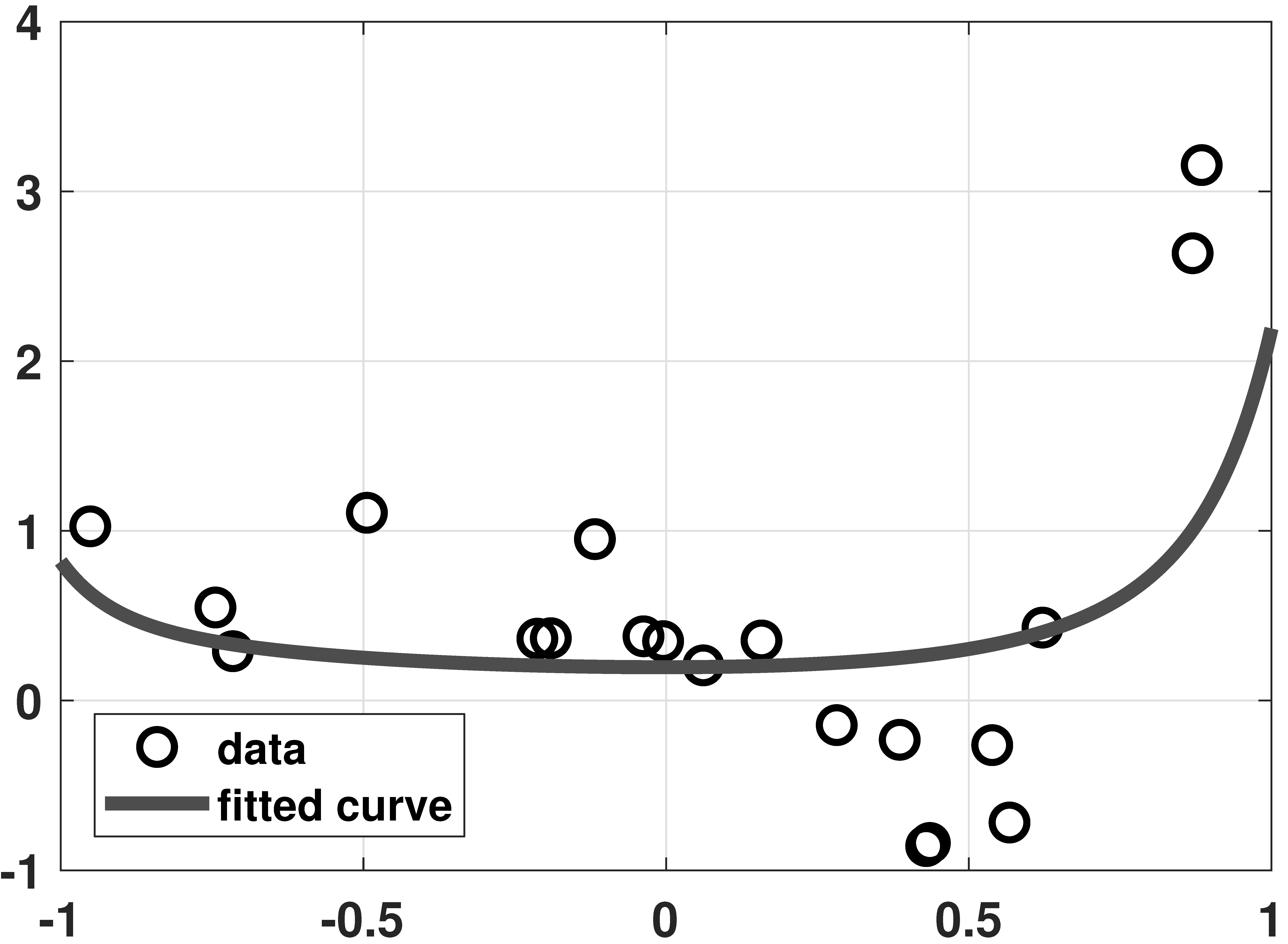
% MATLAB code to demonstrate a ridge regression example
% Generate data
N = 20;
x = linspace(-1,1,N);
a = [0.5, -2, -3, 4, 6];
y = a(1)+a(2)*x(:)+a(3)*x(:).^2+a(4)*x(:).^3+a(5)*x(:).^4+0.25*randn(N,1);

% Ridge regression
lambda = 0.1;
d = 20;
X = zeros(N, d);
for p=0:d-1
    X(:,p+1) = x(:).^p;
end
A = [X; sqrt(lambda)*eye(d)];
b = [y(:); zeros(d,1)];
theta = A\b;

% Interpolate and display results
t    = linspace(-1, 1, 500);
Xhat = zeros(length(t), d);
for p=0:d-1
    Xhat(:,p+1) = t(:).^p;
end
yhat = Xhat*theta;
plot(x,y,   'ko','LineWidth',2, 'MarkerSize', 10); hold on;
plot(t,yhat,'LineWidth',4,'Color',[0.2 0.2 0.9]);

# Python code to demonstrate a ridge regression example
import numpy as np
import matplotlib.pyplot as plt
from scipy.special import eval_legendre
np.set_printoptions(precision=2, suppress=True)

N = 20
x = np.linspace(-1,1,N)
a = np.array([0.5, -2, -3, 4, 6])
y = a[0] + a[1]*x    + a[2]*x**2 + \
           a[3]*x**3 + a[4]*x**4 + 0.2*np.random.randn(N)

d = 20
X = np.zeros((N, d))
for p in range(d):
  X[:,p] = x**p

lambd = 0.1
A = np.vstack((X, np.sqrt(lambd)*np.eye(d)))
b = np.hstack((y, np.zeros(d)))
theta = np.linalg.lstsq(A, b, rcond=None)[0]

t    = np.linspace(-1, 1, 500)
Xhat = np.zeros((500,d))
for p in range(d):
  Xhat[:,p] = t**p
yhat = np.dot(Xhat, theta)

plt.plot(x,y,'o',markersize=12)
plt.plot(t,yhat, linewidth=4)
plt.show()

#  Julia code to demonstrate a ridge regression example

#----------------------------------------------------------
"""
    RidgeRegression(Y,X,lambda,beta0=0)
Calculate ridge regression estimate with targetr vector beta₀.
"""
function RidgeRegression(Y,X,lambda,beta0=0)
    K = size(X,2)
    isa(beta0,Number) && (beta0=fill(beta0,K))
    b = (X'X+lambda*I)\(X'Y+lambda*beta0)      #same as inv(X'X+lambda*I)*(X'Y+lambda*beta0)
    return b
end
#----------------------------------------------------------

N = 20                                 # Generate data
x = range(-1,stop=1,length=N)
a = [0.5, -2, -3, 4, 6]
y = x.^[0 1 2 3 4]*a + 0.25*randn(N)

lambda = 0.1                                # Ridge regression
d = 20
X = x.^collect(0:d-1)'
A = [X; sqrt(lambda)I]
b = [y; zeros(d)]
theta = A\b
theta_alt = RidgeRegression(y,X,lambda)         # alternative ridge regression
display([theta theta_alt])

t    = range(-1,stop=1,length=500)
Xhat = t.^collect(0:d-1)'
yhat = Xhat*theta

p9 = scatter(x,y,markershape=:circle,label="data",legend=:bottomleft)
plot!(t,yhat,linecolor=:blue,linewidth=4,label="fitted curve")
display(p9)

# R code to demonstrate a ridge regression example
N = 20
x = linspace(-1,1,N)
a = c(0.5, -2, -3, 4, 6)
y = a[1] + a[2]*x + a[3]*x**2 + a[4]*x**3 + a[5]*x**4 + 0.2*rnorm(N)

d = 20
X = matrix(0, N, d)
for (p in 1:d) {
  X[,p] = x**p
}
lambd = 0.1
A = rbind(X, (lambd)*diag(d)**(1/2))
b = c(y, rep(0, d))
theta = lsfit(A, b)$coefficients[2:21]

t = linspace(-1, 1, 500)
Xhat = matrix(0, 500,d)
for (p in 1:d) {
  Xhat[,p] = t**p
}
yhat = Xhat %*% theta
plot(x, y)
grid()
lines(t, yhat, col="darkgray", lwd=4)
legend("bottomleft", c("Data", "Fitted curve"), pch=c(1, NA), lty=c(NA, 1))

% MATLAB
data = load('./dataset/ch7_data_crime.txt');
y    = data(:,1);        % The observed crime rate
X    = data(:,3:end);    % Feature vectors
[N,d]= size(X);

lambdaset = logspace(-1,8,50);
theta_store   = zeros(d,50);
for i=1:length(lambdaset)
    lambda = lambdaset(i);
    cvx_begin
        variable theta(d)
        minimize( sum_square(X*theta-y) + lambda*norm(theta,1) )
%       minimize( sum_square(X*theta-y) + lambda*sum_square(theta) )
    cvx_end
    theta_store(:,i) = theta(:);
end

figure(1);
semilogx(lambdaset, theta_store, 'LineWidth', 4);
legend('funding','% high', '% no high', '% college', ...
        '% graduate', 'Location','NW');
xlabel('lambda');
ylabel('feature attribute');

# Python

import cvxpy as cvx
import numpy as np
import matplotlib.pyplot as plt

data = np.loadtxt("/content/ch7_data_crime.txt")
y = data[:,0]
X = data[:,2:7]
N,d = X.shape

lambd_set = np.logspace(-1,8,50)
theta_store = np.zeros((d,50))
for i in range(50):
  lambd = lambd_set[i]
  theta = cvx.Variable(d)
  objective   = cvx.Minimize( cvx.sum_squares(X*theta-y) \
                + lambd*cvx.norm1(theta) )
# objective   = cvx.Minimize( cvx.sum_squares(X*theta-y) \
                + lambd*cvx.sum_squares(theta) )
  prob        = cvx.Problem(objective)
  prob.solve()
  theta_store[:,i] = theta.value

for i in range(d):
  plt.semilogx(lambd_set, theta_store[i,:])

# Julia
"""
    LassoEN(Y,X,lambda,δ,beta₀)
Do Lasso (set lambda>0,δ=0), ridge (set lambda=0,δ>0) or elastic net regression (set lambda>0,δ>0).
Setting beta₀ allows us to specify the target level.
"""
function LassoEN(Y,X,lambda,δ=0.0,beta₀=0)

    K = size(X,2)
    isa(beta₀,Number) && (beta₀=fill(beta₀,K))

    #b_ls = X\Y                    #LS estimate of weights, no restrictions

    Q  = X'X
    c  = X'Y                      #c'b = Y'X*b

    b  = Variable(K)              #define variables to optimize over
    L1 = quadform(b,Q)            #b'Q*b
    L2 = dot(c,b)                 #c'b
    L3 = norm(b-beta₀,1)             #sum(|b-beta₀|)
    L4 = sumsquares(b-beta₀)         #sum((b-beta₀)^2)

    Sol = minimize(L1-2*L2+lambda*L3+δ*L4)      #u'u + lambda*sum(|b|) + δ*sum(b^2), where u = Y-Xb
    solve!(Sol,()->SCS.Optimizer(verbose = false))
    b_i = vec(evaluate(b))

    return b_i

end
#----------------------------------------------------------

using LinearAlgebra, DelimitedFiles, Convex, SCS
import MathOptInterface
const MOI = MathOptInterface

data  = readdlm("dataset/ch7_data_crime.txt")
y     = data[:,1]        # the observed crime rate
X     = data[:,3:end]    # feature vectors
(N,d) = size(X)

(y,X) = (y.-mean(y),X.-mean(X,dims=1))           # de-meaning all variables

lambdaset = exp10.(range(-2,stop=4,length=50))        # adjusted range of lambda values since X/100 is used
(theta_store,theta_store2,theta_store3) = [zeros(50,d) for _=1:3]   # 50 x d instead of d x 50
for i = 1:length(lambdaset)
    theta_store[i,:]  = LassoEN(y/100,X/100,lambdaset[i])    # LASSO, /100 improves the numerical stability
    theta_store2[i,:] = LassoEN(y/100,X/100,0,lambdaset[i])  # ridge regression
    #theta_store3[i,:] = RidgeRegression(y/100,X/100,lambdaset[i])   # alternative ridge regression
end
#display(theta_store2-theta_store3)                                 # compare solutions

p10 = plot(lambdaset,theta_store,xscale=:log10,title="LASSO",xlabel="lambda",ylabel="feature attribute",
           label = ["funding" "% high" "% no high" "% college" "% graduate"],
            linecolor = [:blue :red :yellow3 :magenta :green],ylims=(-5,15))
display(p10)

p10b = plot(lambdaset,theta_store2,xscale=:log10,title="ridge regression",xlabel="lambda",ylabel="feature attribute",
           label = ["funding" "% high" "% no high" "% college" "% graduate"],
            linecolor = [:blue :red :yellow3 :magenta :green],ylims=(-5,15))
display(p10b)

# R
library(pracma)
library(CVXR)

data = scan("ch7_data_crime.txt")
data = matrix(data, nrow=7)
data = t(data)
y = data[,1]
X = data[,3:8]
N = dim(X)[0]
d = dim(X)[1]

lambd_set = logspace(-1,8,50)
theta_store = matrix(0, d,50)
for (i in 1:50) {
  lambd = lambd_set[i]
  theta = Variable(d)
  lambd = lambd_set[i]
  objective = Minimize(sum_squares(X %*% theta-y) 
                         + lambd*norm1(theta))
  # objective   = cvx.Minimize( cvx.sum_squares(X*theta-y) \
  prob = Problem(objective)
  result = solve(prob)
  theta_store[,i] = result$getValue(theta)
}
plot(NULL, xlim=c(10**(-2), 10**8), ylim=c(-2,14))
for (i in 1:d) {
  lines(log(lambd_set), theta_store[i,])
}

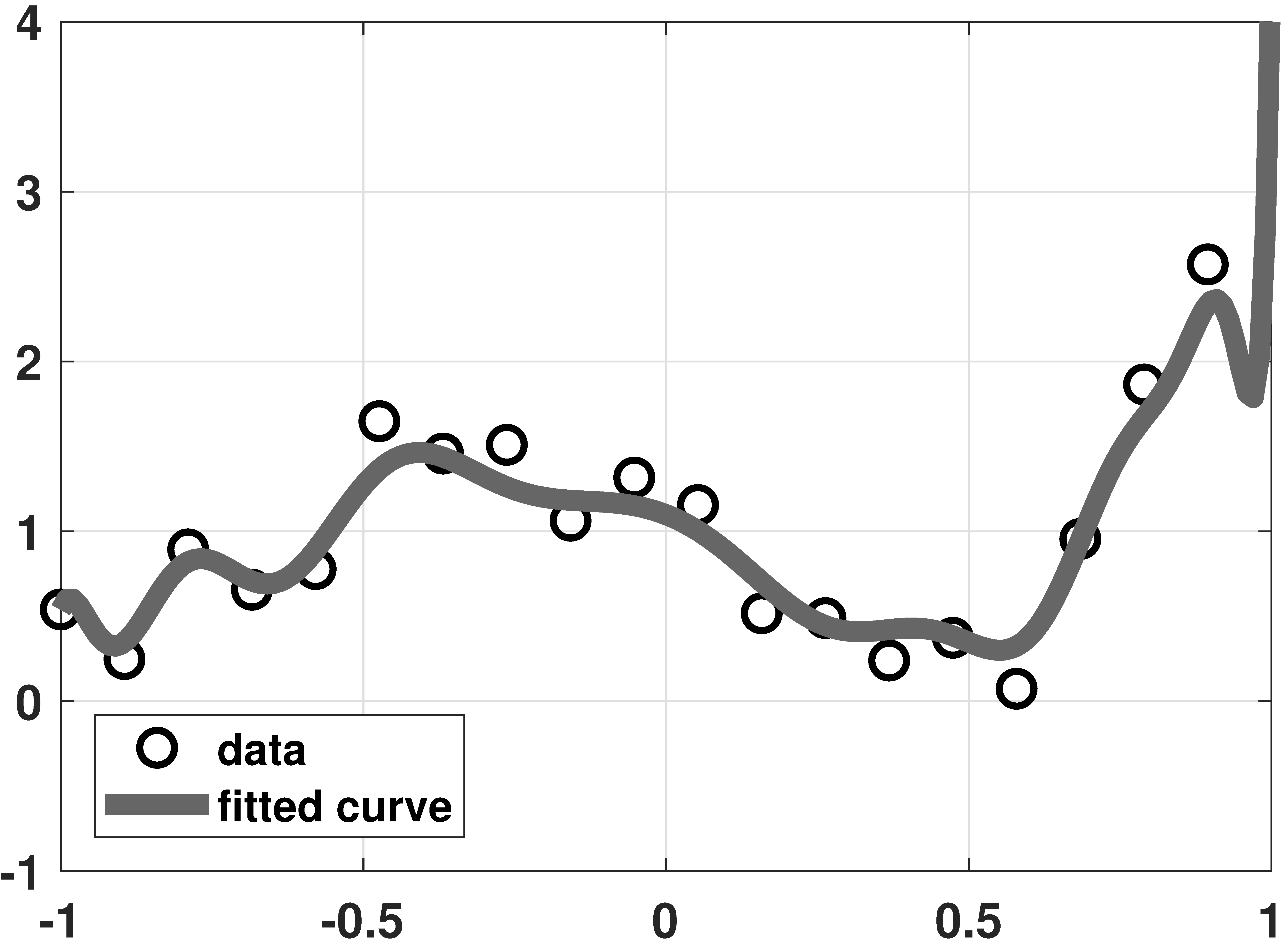
% MATLAB code to demonstrate overfitting and LASSO
% Generate data
N = 20;
x = linspace(-1,1,N)';
a = [1, 0.5, 0.5, 1.5, 1];
y = a(1)*legendreP(0,x)+a(2)*legendreP(1,x)+a(3)*legendreP(2,x)+ ...
    a(4)*legendreP(3,x)+a(5)*legendreP(4,x)+0.25*randn(N,1);

% Solve LASSO using CVX
d = 20;
X = zeros(N, d);
for p=0:d-1
    X(:,p+1) = reshape(legendreP(p,x),N,1);
end
lambda = 2;
cvx_begin
    variable theta(d)
    minimize( sum_square( X*theta - y ) + lambda * norm(theta , 1) )
cvx_end

% Plot results
t    = linspace(-1, 1, 200);
Xhat = zeros(length(t), d);
for p=0:d-1
    Xhat(:,p+1) = reshape(legendreP(p,t),200,1);
end
yhat = Xhat*theta;
plot(x,y,   'ko','LineWidth',2, 'MarkerSize', 10); hold on;
plot(t,yhat,'LineWidth',6,'Color',[0.2 0.5 0.2]);

# Python code to demonstrate overfitting and LASSO
import cvxpy as cvx
import numpy as np
import matplotlib.pyplot as plt

# Setup the problem
N = 20
x = np.linspace(-1,1,N)
a = np.array([1, 0.5, 0.5, 1.5, 1])
y = a[0]*eval_legendre(0,x) + a[1]*eval_legendre(1,x) + \
    a[2]*eval_legendre(2,x) + a[3]*eval_legendre(3,x) + \
    a[4]*eval_legendre(4,x) + 0.25*np.random.randn(N)

# Solve LASSO using CVX
d = 20
lambd = 1
X = np.zeros((N, d))
for p in range(d):
  X[:,p] = eval_legendre(p,x)

theta       = cvx.Variable(d)
objective   = cvx.Minimize( cvx.sum_squares(X*theta-y) \
                            + lambd*cvx.norm1(theta) )
prob        = cvx.Problem(objective)
prob.solve()
thetahat = theta.value

# Plot the curves
t = np.linspace(-1, 1, 500)
Xhat = np.zeros((500,d))
for p in range(P):
  Xhat[:,p] = eval_legendre(p,t)
yhat = np.dot(Xhat, thetahat)
plt.plot(x, y, 'o')
plt.plot(t, yhat, linewidth=4)

# Julia code to demonstrate overfitting and LASSO

using LinearAlgebra, LegendrePolynomials, Convex, SCS
import MathOptInterface
const MOI = MathOptInterface

N = 20                                          # Generate data
x = range(-1,stop=1,length=N)
a = [1, 0.5, 0.5, 1.5, 1]
y = hcat([Pl.(x,p) for p=0:4]...)*a + 0.25*randn(N)

d = 20                                          # Solve LASSO using Convex.jl
X = hcat([Pl.(x,p) for p=0:d-1]...)
lambda = 2
theta = LassoEN(y,X,lambda)

t    = range(-1,stop=1,length=200)
Xhat = hcat([Pl.(t,p) for p=0:d-1]...)
yhat = Xhat*theta

p11 = scatter(x,y,markershape=:circle,label="data",legend=:bottomleft)
plot!(t,yhat,linecolor=:blue,linewidth=4,label="fitted curve")
display(p11)

# R code to demonstrate overfitting and LASSO

# Setup the problem

install.packages("CVXR")
library(pracma)
library(CVXR)

N = 20
x = linspace(-1,1,N)
a = c(1, 0.5, 0.5, 1.5, 1)
y = a[1]*legendre(0,x) + a[2]*legendre(1,x)[1,] +
  a[3]*legendre(2,x)[1,] + a[4]*legendre(3,x)[1,] +
  a[5]*legendre(4,x)[1,] + 0.25*rnorm(N)

# Solve LASSO using CVX
d = 20
lambd = 1
X = matrix(0, N, d)
for (p in 1:d) {
  X[,p] = legendre(p,x)[1,]
}
theta = Variable(d)
objective = Minimize(sum_squares(X %*% theta-y)
                      + lambd*norm1(theta))
prob = Problem(objective)
result = solve(prob)
thetahat = result$getValue(theta)

# Plot the curves
t = linspace(-1, 1, 500)
Xhat = matrix(0, 500, d)
for (p in 1:P) {
  Xhat[,p] = legendre(p,t)[1,]
}
yhat = Xhat %*% thetahat
plot(x, y)
lines(t, yhat)

% MATLAB: Visualize the likelihood function
N = 50;
S = 1:N;
theta = linspace(0.1,0.9,100);
[S_grid, theta_grid] = meshgrid(S, theta);
L = S_grid.*log(theta_grid) + (N-S_grid).*log(1-theta_grid);
s = surf(S,theta,L);
s.LineStyle = '-';
colormap jet
view(65,15)
set(gcf, 'Position', [100, 100, 800, 800]);
set(gca,'FontWeight','bold','fontsize',14);

figure;
N = 50;
S = 1:0.1:N;
theta = linspace(0.1,0.9,1000);
[S_grid, theta_grid] = meshgrid(S, theta);
L = S_grid.*log(theta_grid) + (N-S_grid).*log(1-theta_grid);
imagesc(S,theta,L);
set(gcf, 'Position', [100, 100, 800, 800]);
set(gca,'FontWeight','bold','fontsize',14);
colormap jet

# Python code: Visualizing the likelihood function
import numpy as np
import matplotlib.pyplot as plt
N = 50
S = np.arange(1, N + 1)
theta = np.linspace(0.1, 0.9, 100)
S_grid, theta_grid = np.meshgrid(S, theta)
L = S_grid*np.log(theta_grid) + (N - S_grid)*np.log(1 - theta_grid)
fig = plt.figure()
ax = fig.add_subplot(111, projection='3d')
ax.plot_surface(S_grid, theta_grid, L, cmap='jet')
ax.set_xlabel('S'); ax.set_ylabel('theta'); ax.view_init(15, 65)
plt.figure()
plt.imshow(L, extent=[S.min(), S.max(), theta.min(), theta.max()],
           origin='lower', aspect='auto', cmap='jet')
plt.xlabel('S'); plt.ylabel('theta'); plt.show()

# Julia: Visualizing the likelihood function
using Plots
N = 50
S = range(1., N, step=0.1)
theta = range(0.1, 0.9,length=100)
L(S, theta) = S*log(theta) + (N-S)*log(1. - theta)
# the surface plot
plotlyjs() # this backend allows rotating with mouse
p1 = surface(S, theta, (S, theta) -> L(S, theta), color=:jet, xlabel="S", ylabel="theta",
    title="L(theta|S)") 
# the bird's eye view
gr()
p2 = heatmap(S, theta, (S, theta) -> L(S, theta), color=:jet, xlabel="S", ylabel="theta",
    title="bird's eye view")
SS = 25 # set the value for the slice here
vline!([SS], label=false, color=:black)
# slice through the log likelihood 
p3 = plot(theta, theta -> L(SS, theta),label=false, xlabel="theta", title="L(theta|S=$SS)") 
plot(p2, p3)

# R: Visualize the likelood function
library(pracma)
library(plot3D)

N = 50
S = 1:N
theta = seq(0.1, 0.9, (0.9+0.1)/100)
mesh = meshgrid(S, theta)
S_grid = mesh$X
theta_grid = mesh$Y
L = S_grid * log(theta_grid) + (N-S_grid) * log(1-theta_grid)
L = t(L)
persp3D(S, theta, L, theta=65, phi=15, border="black", lwd=0.3, bty="b2", xlab="S", ylab="θ", zlab="", ticktype="detailed")

# Slice through the log likelihood
N = 50
S = seq(from=1, to=N, by=0.1)
theta = seq(0.1, 0.9, (0.1+0.9)/1000)
mesh = meshgrid(S, theta)
S_grid = mesh$X
theta_grid = mesh$Y
L = S_grid * log(theta_grid) + (N-S_grid) * log(1-theta_grid)
L = t(L)
image(S, theta, L, col=rainbow(256), ylim=c(0.9, 0.1))

% MATLAB code
N = 50;
S = 1:N;
theta = linspace(0.1,0.9,100);
[S_grid, theta_grid] = meshgrid(S, theta);
L = S_grid.*log(theta_grid) + (N-S_grid).*log(1-theta_grid);

figure;
plot(theta, L(:,12), 'LineWidth', 6, 'Color', [0,0,0]);
xlabel('theta');
axis([0.1 0.9 min(ylim) max(ylim)]);
grid on;
set(gcf, 'Position', [100, 100, 600, 400]);
set(gca,'FontWeight','bold','fontsize',14);

# Python code: slice through the likelihood
import numpy as np
import matplotlib.pyplot as plt
N = 50
S = np.arange(1, N + 1)
theta = np.linspace(0.1, 0.9, 100)
S_grid, theta_grid = np.meshgrid(S, theta)
L = S_grid*np.log(theta_grid) + (N - S_grid)*np.log(1 - theta_grid)
plt.plot(theta, L[:, 11], linewidth=6, color='k')   # the column S = 12
plt.xlabel('theta'); plt.grid(True); plt.show()

# Julia code: slice through the likelihood
using Plots
N = 50
theta = range(0.1, 0.9, length=100)
S = 12
L(theta) = S*log(theta) + (N - S)*log(1 - theta)
plot(theta, L.(theta), linewidth=6, color=:black, legend=false,
     xlabel="theta", title="L(theta | S = 12)")

# R code
library(pracma)

N = 50
S = 1:N
theta = seq(0.1, 0.9, (0.1+0.9)/100)
mesh = meshgrid(S, theta)
S_grid = mesh$X
theta_grid = mesh$Y
L = S_grid * log(theta_grid) + (N-S_grid) * log(1-theta_grid)
L_df = data.frame(L)
colnames(L_df) = S

plot(theta, L_df$"12", type="n")
grid()
lines(theta, L_df$"12", lwd=6)
title(expression(paste("L(", theta, " | S = 12)")))

% MATLAB code
lambda = im2double(imread('cameraman.tif'));
T = 100;
x = poissrnd( repmat(lambda, [1,1,T]) );
y = (x>=1);
lambdahat = -log(1-mean(y,3));

figure(1);
imshow(x(:,:,1));

figure(2);
imshow(lambdahat,[]);

# Python code
import cv2
import numpy as np
import scipy.stats as stats
import matplotlib.pyplot as plt
lambd = cv2.imread('./cameraman.tif')               # read image
lambd = cv2.cvtColor(lambd, cv2.COLOR_BGR2GRAY)/255 # gray scale
T = 100
lambdT = np.repeat(lambd[:, :, np.newaxis], T, axis=2)  # repeat image
x = stats.poisson.rvs(lambdT)                       # Poisson statistics
y = (x>=1).astype(float)                            # binary truncation
lambdhat = -np.log(1-np.mean(y,axis=2))             # ML estimation
plt.imshow(lambdhat,cmap='gray')

# Julia: ML estimation for single-photon imaging
using Images, Distributions
using ImageView:imshow
download("https://probability4datascience.com/data/cameraman.tif", "./cameraman.tif")
lambda  = Float64.(load("cameraman.tif"))
T = 100
x = [rand.(Poisson.(lambda)) for _=1:T]
y = [x[i] .>= 1. for i=1:T]
lambdahat = -log.(1. .- mean(y))
imshow(x[1]) # a single sample image
imshow(lambdahat) # the ML recovered image

# R code
library(imager)
lambda = as.data.frame(load.image("cameraman.tif"))
lambda = xtabs(value ~ x+y, data=lambda)
T = 100
x = c()
for (i in 1:T) { 
    x = append(x, rpois(length(lambda), lambda))
}
x = array(x, c(256, 256, T))
y = (x>=1)
mu = apply(y, c(1,2), mean)
lambdahat = -log(1-mu)
fig1 = x[,,1]

# Flip matrix since `image()` reads the matrix bottom up
flip_matrix = function(m) m[,nrow(m):1]

# Figure 1: A single sample image
image(flip_matrix(fig1), col=gray.colors(255))

# Figure 2: ML Recovered Image
image(flip_matrix(lambdahat), col=gray.colors(255))

% MATLAB code
figure;
N = 50;
S = 20;
theta = linspace(0.1,0.9,1000);
L = S.*log(theta) + (N-S).*log(1-theta);
plot(theta, L, 'LineWidth', 6, 'Color', [0.5,0.5,0.75]);
set(gcf, 'Position', [100, 100, 600, 300]);
set(gca,'FontWeight','bold','fontsize',14);
grid on;


h_theta = -log(1-theta);
figure;
plot( theta, h_theta, 'LineWidth', 6, 'Color', [0,0,0]);
set(gcf, 'Position', [100, 100, 600, 400]);
set(gca,'FontWeight','bold','fontsize',14);
grid on;

theta = linspace(0.1,2.5,1000);
L = S.*log(1-exp(-theta)) - theta.*(N-S);
figure;
plot(theta, L, 'LineWidth', 6, 'Color', [0,0,0.75]);
set(gcf, 'Position', [100, 100, 600, 400]);
set(gca,'FontWeight','bold','fontsize',14);
grid on;

# Python code: Visualizing the invariance principle
import numpy as np
import matplotlib.pyplot as plt
N, S = 50, 20
theta = np.linspace(0.1, 0.9, 1000)
L = S*np.log(theta) + (N - S)*np.log(1 - theta)
plt.figure(); plt.plot(theta, L, linewidth=6, color=(0.5, 0.5, 0.75)); plt.grid(True)
h_theta = -np.log(1 - theta)
plt.figure(); plt.plot(theta, h_theta, linewidth=6, color='k'); plt.grid(True)
theta2 = np.linspace(0.1, 2.5, 1000)
L2 = S*np.log(1 - np.exp(-theta2)) - theta2*(N - S)
plt.figure(); plt.plot(theta2, L2, linewidth=6, color=(0, 0, 0.75)); plt.grid(True)
plt.show()

# Julia: Visualizing the invariance principle
using Plots
N = 50
S = 20
theta = range(0.1,0.9,length=1000)
eta  = -log.(1. .- theta) # the reparameterization transformation
L(theta) = S*log(theta) + (N-S)*log(1. - theta) # log likelihood in terms of theta 
L(eta) = S*log(1. - exp(-eta)) - (N-S)*eta # log likelihood in terms of eta 
# plot the log likelihood with theta parameterization 
p4 = plot(theta, theta -> L(theta), linewidth=5, color=:blue, label=false)
xlabel!("theta")
title!("L(theta|S=$S)") 
vline!([0.4], label=false, color=:red)
# plot the transformation
p2 = plot(theta, eta, linewidth=5, color=:black, label=false)
xlabel!("theta")
ylabel!("eta") 
title!("eta(theta)") 
vline!([0.4], label=false, color=:red)
hline!([0.5], label=false, color=:green)
# plot the log likelihood with eta parameterization
p1 = plot(L.(eta), eta,  linewidth=5, color=:blue, label=false, xflip=true)
ylabel!("eta") 
hline!([0.5], label=false, color=:green)
title!("L(eta|S=$S)")
# blank place holder plot
p3 = plot(grid=false, xaxis=false, yaxis=false, xticks=false, yticks=false)
# plot the whole set in the final image
plot(p1, p2, p3, p4)

# R code
N = 50
S = 20
theta = seq(0.1, 0.9, (0.1+0.9)/1000)
L = S * log(theta) + (N-S) * log(1-theta)
plot(theta, L, type="n", xlab=expression(theta), ylab=expression(paste("Log L(", theta, "|S = 20)")))
title("Bernoulli")
grid()
lines(theta, L, lwd=6, col="#8080BF")

h_theta = -log(1-theta)
plot(theta, h_theta, type="n", xlab=expression(theta), ylab=expression(paste(eta, " = h(", theta, ")")))
grid()
lines(theta, h_theta, lwd=6)

theta = seq(0.1, 2.5, (0.1+2.5)/1000)
L = S * log(1-exp(-theta)) - theta * (N-S)
plot(theta, L, type="n")
title("Truncated Poisson")
grid()
lines(theta, L, lwd=6, col="#0000BF")

% MATLAB code
N = 1;
sigma0 = 1;
mu0    = 0.0;
x = 5;%*rand(N,1);
t = linspace(-3,7,1000);

q = NaN(1,1000);
for i=1:N
    [val,idx] = min(abs(t-x(i)));
    q(idx) = 0.1;
end

p0 = normpdf(t,0,1);
theta = (mean(x)*sigma0^2+mu0/N)/(sigma0^2+1/N);
p1 = normpdf(t,theta,1);
prior = normpdf(t,mu0,sigma0)/10;

figure;
h1 = plot(t,normpdf(t,mean(x),1),'LineWidth',4,'Color',[0.8,0.8,0.8]); hold on; 
h2 = plot(t,p1,'LineWidth',4,'Color',[0,0.0,0.0]);
h3 = stem(t,q,'LineWidth',4,'Color',[0.5,0.5,0.5],'MarkerSize',10); 
h5 = plot(t,prior,'LineWidth',4,'Color',[1,0.5,0.0]);

grid on;
axis([-3 7 0 0.5]);
xticks(-5:1:10);
yticks(0:0.05:0.5);
set(gcf, 'Position', [100, 100, 600, 300]);
set(gca,'FontWeight','bold','fontsize',14);

# Python code: Influence of the priors
import numpy as np
import matplotlib.pyplot as plt
from scipy.stats import norm
N = 5
mu0, sigma0 = 0.0, 1.0
theta_true = 5.0
x = np.random.normal(theta_true, 1, N)
xbar = np.mean(x)
t = np.linspace(-3, 7, 1000)
thetahat = (sigma0**2*xbar + mu0/N)/(sigma0**2 + 1/N)
sigmahat = np.sqrt(1/(1/sigma0**2 + N))
plt.plot(t, norm.pdf(t, xbar, 1.0), linewidth=3, label='Likelihood')
plt.plot(t, norm.pdf(t, thetahat, sigmahat), linewidth=3, label='Posterior')
plt.plot(t, norm.pdf(t, mu0, sigma0), linewidth=3, label='Prior')
plt.stem(x, 0.1*np.ones(N), linefmt='gray', markerfmt='o', basefmt=' ', label='data')
plt.legend(); plt.title(f'N = {N}'); plt.show()

# Julia: Influence of the priors
# likelihood is N(theta,1) 
using Plots, Distributions
N = 5       # sample size
mu0  = 0.0   # prior mean
sigma0  = 1.    # prior std. dev.
theta = 5.      # true mean of sample data
x = rand(Normal(theta,1), N)    # the sample data
xbar  = mean(x) # mean of sample data
t = range(-3.,7.,length=1000)
thetahat = (sigma0^2. * xbar + mu0/N)/(sigma0^2. + 1. /N) # MAP
sigmahat = sqrt(1. / (1. / sigma0^2. + N))  # s.d. posterior 
p0 = pdf(Normal(xbar,1.0), t)       # likelihood
p1 = pdf(Normal(thetahat, sigmahat), t)  # posterior
prior = pdf(Normal(mu0,sigma0),t)     # prior, divided by 10 to 
plot(t, [p0, p1, prior], label=["Likelihood" "Posterior" "prior"], linewidth=3, legend=:topleft)
plot!([x], [0.1*ones(N)], line=:stem, label="data", marker=:circle, linewidth=3, title="N = $N")

# R code: Influence of the priors
N = 5
mu0 = 0.0
sigma0 = 1
theta = 5
x = rnorm(N, 5, 1)
xbar = mean(x)
t = seq(-3, 7, (10)/1000)
q = numeric(1000)
for (i in 1:N) {
    x = abs(t-x[i])
    a = min(x)
    q[match(a, x)] = 0.1 
}
thetahat = (sigma0^2. * xbar + mu0/N)/(sigma0^2. + 1. /N)
sigmahat = sqrt(1. / (1. / sigma0^2 + N))
p0 = dnorm(t, xbar, 1.)
p1 = dnorm(t, thetahat, sigmahat)
prior = dnorm(t, mu0, sigma0)/10
plot(t, p1, type="n")
title("N = 5")
legend(-2, 0.9, legend=c("Likelihood", "Posterior", "Prior", "Data"), col=c("blue", "orange", "green", "purple"), lty=1:1)
grid()
lines(t, p0, lwd = 4, col="blue")
lines(t, p1, lwd = 4, col="orange")
lines(t, prior, lwd = 4, col="green")
lines(t, q, lwd = 4, col="purple")
grid()

% MATLAB code
sigma0 = 0.25;
mu0    = 0.0;

mu     = 1;
sigma  = 0.25;

Nset = [0 1 2 5 8 12 20];
x0 = sigma*randn(100,1);

for i=1:7
    N = Nset(i);
    x = x0(1:N);
    t = linspace(-1,1.5,1000);
    
    p0     = normpdf(t,0,1);
    theta  = mu*(N*sigma0^2)/(N*sigma0^2+sigma^2) + mu0*(sigma^2)/(N*sigma0^2+sigma^2);
    sigmaN = sqrt(1/(1/sigma0^2+N/sigma^2));
    posterior(:,i) = normpdf(t,theta,sigmaN);
end

figure;
plot(t,posterior(:,1)', 'LineWidth',2,'Color',[0.9,0.0,0.0]);  hold on;
plot(t,posterior(:,2)', 'LineWidth',2,'Color',[1,0.6,0.0]);
plot(t,posterior(:,3)', 'LineWidth',2,'Color',[1,0.9,0.3]);
plot(t,posterior(:,4)', 'LineWidth',2,'Color',[0.0,0.8,0.1]); 
plot(t,posterior(:,5)', 'LineWidth',2,'Color',[0.0,0.6,0.6]); 
plot(t,posterior(:,6)', 'LineWidth',2,'Color',[0.0,0.2,0.8]); 
plot(t,posterior(:,7)', 'LineWidth',2,'Color',[0.5,0.2,0.5]); 

legend('N = 0', 'N = 1', 'N = 2', 'N = 5', 'N = 8', 'N = 12', 'N = 20', 'Location', 'NW');
grid on;
axis([-1 1.5 0 8]);
set(gcf, 'Position', [100, 100, 600, 300]);
set(gca,'FontWeight','bold','fontsize',14);

# Python code: Conjugate priors
import numpy as np
import matplotlib.pyplot as plt
from scipy.stats import norm
sigma0, mu0 = 0.25, 0.0
mu, sigma = 1.0, 0.25
Nset = [0, 1, 2, 5, 8, 12, 20]
t = np.linspace(-1, 1.5, 1000)
colors = [(0.9,0,0),(1,0.6,0),(1,0.9,0.3),(0,0.8,0.1),(0,0.6,0.6),(0,0.2,0.8),(0.5,0.2,0.5)]
for N, c in zip(Nset, colors):
    theta  = mu*(N*sigma0**2)/(N*sigma0**2 + sigma**2) + mu0*(sigma**2)/(N*sigma0**2 + sigma**2)
    sigmaN = np.sqrt(1/(1/sigma0**2 + N/sigma**2))
    plt.plot(t, norm.pdf(t, theta, sigmaN), linewidth=2, color=c, label=f'N = {N}')
plt.legend(loc='upper left'); plt.axis([-1, 1.5, 0, 8]); plt.grid(True); plt.show()

% Julia
using Plots, Distributions
sigma0 = 0.25
mu0 = 0.0
mu  = 1.
sigma  = 0.25
Nset = [0 1 2 5 8 12 20]
x0 = sigma .* randn(100)
posterior = zeros(1000,7)
t = range(-1.,1.5,length=1000)
p0 = pdf(Normal(0.,1.), t)
for i=1:7
    N = Nset[i]
    x = x0[1:N]
    theta  = mu * (N*sigma0^2.)/(N*sigma0^2. + sigma ^2.) + mu0*(sigma^2.)/(N*sigma0^2. + sigma^2.)
    sigmaN= sqrt(1. /(1. /sigma0^2. + N/sigma^2.))
    posterior[:,i] = pdf(Normal(theta, sigmaN), t)
end
plot(t, posterior, linewidth=2., 
    label=["N = 0" "N = 1" "N = 2" "N = 5" "N = 8" "N = 12" "N = 20"],
    legend=:topleft)

# R code
sigma0 = 0.25
mu0 = 0.0
mu = 1
sigma = 0.25
Nset = c(0, 1, 2, 5, 8, 12, 20)
x0 = sigma * rnorm(100)
posterior = list()
for (i in 1:7) {
    N = Nset[i]
    x = x0[1:N]
    t = seq(-1, 1.5, 2.5/1000)
    p0 = dnorm(t, 0, 1)
    theta = mu*(N*sigma0^2)/(N*sigma0^2+sigma^2) + mu0*(sigma^2)/(N*sigma0^2+sigma^2)
    sigmaN = sqrt(1/(1/sigma0^2+N/sigma^2));
    posterior[[i]] = dnorm(t, theta, sigmaN)
}

plot(t, posterior[[7]], type="n", xlab="", ylab="")
grid()
lines(t, posterior[[1]], lwd=3, col="red")
lines(t, posterior[[2]], lwd=3, col="orange")
lines(t, posterior[[3]], lwd=3, col="yellow")
lines(t, posterior[[4]], lwd=3, col="green")
lines(t, posterior[[5]], lwd=3, col="turquoise")
lines(t, posterior[[6]], lwd=3, col="blue")
lines(t, posterior[[7]], lwd=3, col="purple")

legend(-0.9, 7, legend=c("N = 0", "N = 1", "N = 2", "N = 5", "N = 8", "N = 12", "N = 20"), col=c("red", "orange", "yellow", "green", "turquoise", "blue", "purple"), lty=1:1, lwd=3)
grid()

% MATLAB code
gmm = gmdistribution([0; 5], cat(3,1,1), [0.3 0.7]);
x = linspace(-5, 10, 1000)';
f = pdf(gmm, x);
figure;
plot(x,f,'LineWidth', 6,'color',[0.1, 0.4, 0.6]);
grid on;
axis([-5 10 0 0.35]);
legend('Population', 'Location', 'NW');
set(gcf, 'Position', [100, 100, 600, 300]);
set(gca,'FontWeight','bold','fontsize',14);

for i=1:4
    figure;
    bin = -5:10;
    Y = random(gmm, 50);
    [num,val] = hist(Y,bin);
    bar(val, num,'FaceColor',[0.1, 0.4, 0.6]);
    tt = sprintf('Mean = %3.2f', mean(Y));
    legend(tt, 'Location', 'NW');
    grid on;
    axis([-5 10 0 20]);
    set(gcf, 'Position', [100, 100, 600, 300]);
    set(gca,'FontWeight','bold','fontsize',14);
end

bin = 2:0.1:5;
for i=1:10000
    Y(:,i) = random(gmm, 50);
end
M = mean(Y);
[num,val] = hist(M,bin);
bar(val, num,'FaceColor',[0.2, 0.2, 0.2]);
grid on;
axis([2 5 0 1200]);
set(gcf, 'Position', [100, 100, 600, 300]);
set(gca,'FontWeight','bold','fontsize',14);
legend('Sample Average');

# Python code: Histogram of the sample average
import numpy as np
import matplotlib.pyplot as plt
from scipy.stats import norm
def sample_gmm(n):
    return np.where(np.random.rand(n) < 0.7,
                    np.random.normal(5, 1, n), np.random.normal(0, 1, n))
x = np.linspace(-5, 10, 1000)
f = 0.3*norm.pdf(x, 0, 1) + 0.7*norm.pdf(x, 5, 1)
plt.figure(); plt.plot(x, f, linewidth=6, color=(0.1, 0.4, 0.6)); plt.legend(['Population'])
for i in range(4):
    plt.figure()
    Y = sample_gmm(50)
    plt.hist(Y, bins=np.arange(-5, 11), color=(0.1, 0.4, 0.6))
    plt.legend([f'Mean = {np.mean(Y):.2f}'])
M = np.array([np.mean(sample_gmm(50)) for _ in range(10000)])
plt.figure(); plt.hist(M, bins=np.arange(2, 5.01, 0.1), color=(0.2, 0.2, 0.2))
plt.legend(['Sample Average']); plt.show()

# Julia: Histogram of the sample average
using Distributions, Plots, Printf
gmm = MixtureModel(Normal[Normal(), Normal(5., 1.),], [0.3, 0.7])
x = range(-5., 10., length=1000)
# the population distribution
plot(x, pdf(gmm, x), linewidth=3, label=false, title="Population distribution")
# histograms of 4 random samples of size 50
plot_array = [] 
for i=1:4
    bin = -5:10
    Y = rand(gmm, 50)
    tt = @sprintf("Mean = %3.2f", mean(Y))
    push!(plot_array, histogram(Y, bins=bin, label = tt, legend=:topleft))
end
plot(plot_array...)
# histogram of sample average
M = zeros(10000)
bin = range(2., 5., step=0.1)
for i = 1:10000
    M[i] = mean(rand(gmm, 50))
end   
histogram(M, bins=bin, label=false, title="Histogram of the sample average")

# R code: Histogram of the sample average
sample_gmm <- function(n) ifelse(runif(n) < 0.7, rnorm(n, 5, 1), rnorm(n, 0, 1))
x <- seq(-5, 10, length.out=1000)
f <- 0.3*dnorm(x, 0, 1) + 0.7*dnorm(x, 5, 1)
plot(x, f, type="l", lwd=6, col=rgb(0.1, 0.4, 0.6), ylim=c(0, 0.35))
legend("topleft", "Population", lwd=6, col=rgb(0.1, 0.4, 0.6))
for (i in 1:4) {
    Y <- sample_gmm(50)
    hist(Y, breaks=seq(-5, 10, 1), col=rgb(0.1, 0.4, 0.6),
         main=sprintf("Mean = %3.2f", mean(Y)))
}
M <- replicate(10000, mean(sample_gmm(50)))
hist(M, breaks=seq(2, 5, 0.1), col="gray20", main="Sample Average")

% MATLAB code to compute the width of the confidence interval
alpha = 0.05;
mu = 0; sigma = 1; % Standard Gaussian
epsilon = icdf('norm',1-alpha/2,mu,sigma)

# Python code to compute the width of the confidence interval
import scipy.stats as stats
alpha = 0.05;
mu   = 0; sigma = 1; # Standard Gaussian
epsilon = stats.norm.ppf(1-alpha/2, mu, sigma)
print(epsilon)

# Julia code to compute the width of the confidence interval
using Distributions
alpha = 0.05
mu = 0.
sigma = 1.
epsilon = quantile(Normal(mu, sigma ), 1. - alpha/2.) # CI is estimator ± epsilon

# R: Histogram of the sample average
alpha = 0.05
mu = 0
sigma = 1
epsilon = qnorm(0.975, mu, sigma)
epsilon

% MATLAB code to plot the t-distribution
x = linspace(-5,5,100);
p1 = pdf('norm',x,0,1);
p2 = pdf('t',x,11-1);
p3 = pdf('t',x,3-1);
p4 = pdf('t',x,2-1);

figure;
plot(x,p1,'-.','LineWidth',4,'Color',[0 0.6 0]); hold on;
plot(x,p2,'-o','LineWidth',2,'Color',[1 0.6 0.2]);
plot(x,p3,'-^','LineWidth',2,'Color',[0.2 0.2 0.7]);
plot(x,p4,'-s','LineWidth',2,'Color',[0.7 0.2 0.2]);
legend('Gaussian(0,1)', 't-dist, N = 11', 't-dist, N = 3', 't-dist, N = 2');
grid on;
xticks(-5:1:5);
yticks(0:0.05:0.4);
set(gcf, 'Position', [100, 100, 600, 300]);
set(gca,'FontWeight','bold','fontsize',14);

# Python code to plot the t-distribution
import numpy as np
import matplotlib.pyplot as plt
from scipy.stats import norm, t
x = np.linspace(-5, 5, 100)
plt.plot(x, norm.pdf(x), '-.', linewidth=4, color=(0, 0.6, 0), label='Gaussian(0,1)')
plt.plot(x, t.pdf(x, 11 - 1), '-o', linewidth=2, color=(1, 0.6, 0.2), label='t-dist, N = 11')
plt.plot(x, t.pdf(x, 3 - 1),  '-^', linewidth=2, color=(0.2, 0.2, 0.7), label='t-dist, N = 3')
plt.plot(x, t.pdf(x, 2 - 1),  '-s', linewidth=2, color=(0.7, 0.2, 0.2), label='t-dist, N = 2')
plt.legend(); plt.grid(True); plt.show()

# Julia code to plot the t-distribution
using Distributions, Plots
x = range(-5.,5.,length=100)
p1 = pdf(Normal(),x)
p2 = pdf(TDist(11-1),x)
p3 = pdf(TDist(3-1),x)
p4 = pdf(TDist(2-1),x)
plot([p1,p2,p3,p4], label = ["Gaussian(0,1)" "t-dist, N = 11" "t-dist, N = 3" "t-dist, N = 2"], legend=:topright)

# R code to plot the t-distribution
x <- seq(-5, 5, length.out=100)
plot(x, dnorm(x), type="l", lty=4, lwd=4, col="darkgreen", ylim=c(0, 0.4),
     xlab="x", ylab="pdf")
lines(x, dt(x, 11 - 1), lwd=2, col="orange")
lines(x, dt(x, 3 - 1),  lwd=2, col="blue")
lines(x, dt(x, 2 - 1),  lwd=2, col="darkred")
legend("topright", c("Gaussian(0,1)", "t-dist, N = 11", "t-dist, N = 3", "t-dist, N = 2"),
       col=c("darkgreen", "orange", "blue", "darkred"), lty=c(4, 1, 1, 1), lwd=2)
grid()

% MATLAB code to generate a confidence interval
x         = [72 69 75 58 67 70 60 71 59 65];
N         = numel(x);
Theta_hat = mean(x);            % Sample mean
S_hat     = std(x);             % Sample standard deviation
nu        = N - 1;              % degrees of freedom
alpha     = 0.05;               % confidence level
z         = tinv(1 - alpha/2, nu);
CI_L      = Theta_hat - z*S_hat/sqrt(N);
CI_U      = Theta_hat + z*S_hat/sqrt(N);
fprintf('Confidence interval: [%5.3f, %5.3f]\n', CI_L, CI_U);

# Python code to generate a confidence interval
import numpy as np
import scipy.stats as stats
x = np.array([72, 69, 75, 58, 67, 70, 60, 71, 59, 65])
N         = x.size     
Theta_hat = np.mean(x) # Sample mean
S_hat     = np.std(x)  # Sample standard deviation
nu        = x.size-1   # degrees of freedom
alpha     = 0.05       # confidence level
z    = stats.t.ppf(1-alpha/2, nu)
CI_L = Theta_hat-z*S_hat/np.sqrt(N)
CI_U = Theta_hat+z*S_hat/np.sqrt(N)
print(CI_L, CI_U)

# Julia code to generate a confidence interval
using Statistics, Distributions, Printf
x = [72., 69., 75., 58., 67., 70., 60., 71., 59., 65.]
thetahat = mean(x)  # Sample mean
sigmahat = std(x)   # Sample standard deviation
N = size(x,1)
nu = N-1 # degrees of freedom
alpha = 0.05        # confidence level
z = quantile(TDist(nu), 1. - alpha/2.)
CI_L = thetahat - z*sigmahat/sqrt(N)
CI_U = thetahat + z*sigmahat/sqrt(N)
@printf("Confidence interval: [%5.3f - %5.3f]", CI_L, CI_U)

# R code to generate a confidence interval
x <- c(72,69,75,58,67,70,60,71,59,65)
N = length(x)
Theta_hat = mean(x)
S_hat = sd(x)
nu = length(x) - 1
alpha = 0.05
z = qt(1-alpha/2, nu)
CI_L = Theta_hat-z*S_hat/sqrt(N)
CI_U = Theta_hat+z*S_hat/sqrt(N)
CI_L
CI_U

% MATLAB code to illustrate bootstrap
gmm = gmdistribution([0; 5], cat(3,1,1), [0.3 0.7]);
x = linspace(-5, 10, 1000)';
f = pdf(gmm, x);
figure;
plot(x,f,'LineWidth', 6,'color',[0.1, 0.4, 0.6]);
grid on;
axis([-5 10 0 0.35]);
legend('Population', 'Location', 'NW');
set(gcf, 'Position', [100, 100, 600, 300]);
set(gca,'FontWeight','bold','fontsize',14);

% Visualize bootstrap dataset
N = 100;
X = random(gmm, N);
figure;
[num,val] = hist(X, linspace(-5,10,30));
bar(val, num,'FaceColor',[0.1, 0.4, 0.6]);
set(gcf, 'Position', [100, 100, 600, 300]);
set(gca,'FontWeight','bold','fontsize',14);

for i=1:3
    % Bootstrap dataset
    idx = randi(N,[1, N]);
    Xb1 = X(idx);
    figure;
    [num,val] = hist(Xb1, linspace(-5,10,30));
    bar(val, num,'FaceColor',[0.1, 0.4, 0.6]);
    set(gcf, 'Position', [100, 100, 600, 300]);
    set(gca,'FontWeight','bold','fontsize',14);
end

% Bootstrap 
K = 1000;
Thetahat = zeros(1,K);
for i=1:K                       % repeat K times
    idx = randi(N,[1, N]);      % sampling w/ replacement
    Y = X(idx);
    Thetahat(i) = median(Y);    % estimator
end
M = mean(Thetahat)              % bootstrap mean
V = var(Thetahat)               % bootstrap variance
figure;
[num,val] = hist(Thetahat, linspace(3.5,5.5,30));
bar(val, num,'FaceColor',[0.2, 0.2, 0.2]);
set(gcf, 'Position', [100, 100, 600, 300]);
set(gca,'FontWeight','bold','fontsize',14);

# Python code to illustrate bootstrap
import numpy as np
import matplotlib.pyplot as plt
def sample_gmm(n):
    return np.where(np.random.rand(n) < 0.7,
                    np.random.normal(5, 1, n), np.random.normal(0, 1, n))
N = 100
X = sample_gmm(N)
plt.figure(); plt.hist(X, bins=np.linspace(-5, 10, 30), color=(0.1, 0.4, 0.6))
for i in range(3):
    idx = np.random.randint(0, N, N)
    plt.figure(); plt.hist(X[idx], bins=np.linspace(-5, 10, 30), color=(0.1, 0.4, 0.6))
K = 1000
thetahat = np.zeros(K)
for i in range(K):
    idx = np.random.randint(0, N, N)   # sampling with replacement
    thetahat[i] = np.median(X[idx])    # estimator
M = np.mean(thetahat)                  # bootstrap mean
V = np.var(thetahat)                   # bootstrap variance
print(M, V)
plt.figure(); plt.hist(thetahat, bins=np.linspace(3.5, 5.5, 30), color=(0.2, 0.2, 0.2))
plt.show()

# Julia code to illustrate bootstrap
using Plots, Distributions, Statistics
gmm = MixtureModel(Normal[Normal(), Normal(5., 1.),], [0.3, 0.7])
# visualize the population
x = range(-5., 10., length=1000);
f = pdf(gmm, x);
plot(x, pdf(gmm,x), linewidth=3, label="Population", legend=:topleft)
# Visualize bootstrap dataset, the real sample data
N = 100
X = rand(gmm, N) # the real sample data
p1 = histogram(X, bins = range(-5,10,length=30), label=false)
# visualize 3 bootstrap samples
plot_array = [] 
for i=1:3
    # Bootstrap dataset
    idx = rand(1:N, N)
    Xb1 = X[idx]
    push!(plot_array, histogram(Xb1, bins = range(-5.,10.,length=30)))
end
plot(plot_array..., label=false)

# Bootstrap the median
K = 1000 # number of bootstrap re-samples
thetahat = zeros(K)
for i=1:K               # repeat K times
    idx = rand(1:N, N)  # sampling w/ replacement
    Y = X[idx]
    thetahat[i] = median(Y) # estimator
end
M = mean(thetahat)          # bootstrap mean
V = var(thetahat)           # bootstrap variance
# histogram of bootstrap replications of estimator
histogram(thetahat, bins=range(3.5,5.5,length=30), legend=false)

# R code to illustrate bootstrap
sample_gmm <- function(n) ifelse(runif(n) < 0.7, rnorm(n, 5, 1), rnorm(n, 0, 1))
N <- 100
X <- sample_gmm(N)
hist(X, breaks=seq(-5, 10, length.out=30), col=rgb(0.1, 0.4, 0.6))
for (i in 1:3) {
    idx <- sample.int(N, N, replace=TRUE)
    hist(X[idx], breaks=seq(-5, 10, length.out=30), col=rgb(0.1, 0.4, 0.6))
}
K <- 1000
thetahat <- numeric(K)
for (i in 1:K) {
    idx <- sample.int(N, N, replace=TRUE)   # sampling with replacement
    thetahat[i] <- median(X[idx])           # estimator
}
M <- mean(thetahat)   # bootstrap mean
V <- var(thetahat)    # bootstrap variance
print(c(M, V))
hist(thetahat, breaks=seq(3.5, 5.5, length.out=30), col="gray20")

% MATLAB code to estimate a bootstrap variance
X = [72, 69, 75, 58, 67, 70, 60, 71, 59, 65];
N = size(X,2);
K = 1000;
Thetahat = zeros(1,K);
for i=1:K                       % repeat K times
    idx = randi(N,[1, N]);      % sampling w/ replacement
    Y = X(idx);
    Thetahat(i) = median(Y);    % estimator
end
M = mean(Thetahat)              % bootstrap mean
V = var(Thetahat)               % bootstrap variance

# Python code to estimate a bootstrap variance
import numpy as np
X = np.array([72, 69, 75, 58, 67, 70, 60, 71, 59, 65])
N = X.size
K = 1000
Thetahat = np.zeros(K)
for i in range(K):
  idx = np.random.randint(N, size=N)
  Y = X[idx]
  Thetahat[i] = np.median(Y)
M = np.mean(Thetahat)
V = np.var(Thetahat)

# Julia code to estimate a bootstrap variance
using Statistics
X = [72., 69., 75., 58., 67., 70., 60., 71., 59., 65.]
N = size(X,1)
K = 1000
thetahat = zeros(K)
for i=1:K                       # repeat K times
    idx = rand(1:N, N)          # sampling w/ replacement
    Y = X[idx]
    thetahat[i] = median(Y)         # estimator
end
M = mean(thetahat)                  # bootstrap mean
V = var(thetahat)                   # bootstrap variance

# R code to estimate a bootstrap variance
X <- c(72, 69, 75, 58, 67, 70, 60, 71, 59, 65)
N = length(X)
K = 1000
Thetahat = rep(0, K)
for (i in 0:K) {
    idx = sample(N,5)
    Y = X[idx]
    Thetahat[i] = median(Y)
}
M = mean(Thetahat)
V = var(Thetahat)
M
V

% MATLAB command to estimate the Z_hat value.
Theta_hat = 0.29;                    % Your estimate
theta    = 0.25;                     % Your hypothesis
sigma    = sqrt(theta*(1-theta));    % Known standard deviation
N        = 1000;                     % Number of samples
Z_hat    = (Theta_hat - theta)/(sigma/sqrt(N));

# Python command to estimate the Z_hat value
import numpy as np
Theta_hat = 0.29                     # Your estimate
theta     = 0.25                     # Your hypothesis
N         = 1000                     # Number of samples
sigma     = np.sqrt(theta*(1-theta)) # Known standard deviation
Z_hat = (Theta_hat - theta)/(sigma / np.sqrt(N))
print(Z_hat)

# Julia Estimate Z-value
thetahat = 0.29                 # Your estimate
theta = 0.25                    # Your hypothesis
sigma = sqrt(theta*(1. - theta))        # Known standard deviation
N = 1000                    # Number of samples
Z_hat = (thetahat - theta)/(sigma/sqrt(N))

# R Estimate Z-value
Theta_hat = 0.29                     # Your estimate
theta     = 0.25                     # Your hypothesis
N         = 1000                     # Number of samples
sigma     = sqrt(theta*(1-theta)) # Known standard deviation
Z_hat = (Theta_hat - theta)/(sigma / sqrt(N))
Z_hat

% MATLAB code to compute the critical value
alpha = 0.05;
z_alpha = icdf('norm', 1-alpha, 0, 1);

# Python code to compute the critical value
import scipy.stats as stats
alpha = 0.05
z_alpha = stats.norm.ppf(1-alpha, 0, 1)

# Julia code to compute the critical value
using Distributions
alpha = 0.05
z_alpha = quantile(Normal(), 1-alpha)

# R code to compute the critical value
alpha = 0.05
z_alpha = qnorm(1-alpha, 0, 1)
z_alpha

% MATLAB code to compute the p-value
p = cdf('norm', -1.92, 0, 1);

# Python code to compute the p-value
import scipy.stats as stats
p = stats.norm.cdf(-1.92,0,1)

# Julia code to compute the p-value
using Distributions
p = cdf(Normal(), -1.92)

# R code to compute the p-value
p = pnorm(-1.92,0,1)
p

% MATLAB code to plot ROC curve
sigma = 2;  mu = 3;
alphaset = linspace(0,1,1000);
PF1 = zeros(1,1000); PD1 = zeros(1,1000);
PF2 = zeros(1,1000); PD2 = zeros(1,1000);
for i=1:1000
    alpha = alphaset(i);
    PF1(i) = alpha;
    PD1(i) = alpha;

    PF2(i) = alpha;
    PD2(i) = 1-normcdf(norminv(1-alpha)-mu/sigma);
end
figure;
plot(PF1, PD1,'LineWidth', 4, 'Color', [0.8, 0, 0]); hold on;
plot(PF2, PD2,'LineWidth', 4, 'Color', [0, 0, 0]); hold off;

# Python code to plot ROC curve
import numpy as np
import matplotlib.pyplot as plt
import scipy.stats as stats

sigma = 2; mu = 3;
alphaset = np.linspace(0,1,1000)
PF1 = np.zeros(1000); PD1 = np.zeros(1000)
PF2 = np.zeros(1000); PD2 = np.zeros(1000)
for i in range(1000):
  alpha = alphaset[i]
  PF1[i] = alpha
  PD1[i] = alpha
  PF2[i] = alpha
  PD2[i] = 1-stats.norm.cdf(stats.norm.ppf(1-alpha)-mu/sigma)
plt.plot(PF1,PD1)
plt.plot(PF2,PD2)

# Julia code to plot ROC curve
using Distributions, Plots, Statistics
sigma = 2.
mu = 3.
PF1 = zeros(1000); PD1 = zeros(1000)
PF2 = zeros(1000); PD2 = zeros(1000)
alphaset = range(0.,1.,length=1000)
d = Normal()
for i=1:1000
    alpha = alphaset[i]
    PF1[i] = alpha
    PD1[i] = alpha
    PF2[i] = alpha
    PD2[i] = 1. - cdf(d, quantile(d, 1-alpha)-mu/sigma)
end
plot(PF1, PD1, linewidth=3, label = "Blind guess")
plot!(PF2, PD2, linewidth=3, label = "Neyman-Pearson", legend=:bottomright)

# R code to plot ROC curve
#install.packages("matlab", repo="http://cran.r-project.org", dep=T)
library(matlab)

sigma = 2 
mu = 3
alphaset <- linspace(0,1,1000)
PF1 = rep(0, 1000) 
PD1 = rep(0, 1000)
PF2 = rep(0, 1000)
PD2 = rep(0, 1000)
for (i in 0:1000) {
    alpha = alphaset[i]
    PF1[i] = alpha
    PD1[i] = alpha
    PF2[i] = alpha
    PD2[i] = 1-pnorm(qnorm(1-alpha)-mu/sigma)
}

#roc_plot <- rbind(, plot(PF2,PD2))
#roc_plot
plot(PF1,PD1,type = "l", col = "red")
lines(PF2, PD2, col = "black")

% MATLAB
auc1 = sum(PD1.*[0 diff(PF1)])
auc2 = sum(PD2.*[0 diff(PF2)])

# Python
auc1 = np.sum(PD1 * np.append(0, np.diff(PF1)))
auc2 = np.sum(PD2 * np.append(0, np.diff(PF2)))

# Julia
# Computer area under curve
auc1 = sum(PD1.*[0.; diff(PF1)])
auc2 = sum(PD2.*[0.; diff(PF2)])

# R
auc1 = sum(PD1 * c(0, diff(PF1)))
auc2 = sum(PD2 * c(0, diff(PF2)))
auc1
auc2

% MATLAB code to generate the ROC curve.
sigma = 2;  mu = 3;
PF1 = zeros(1,1000); PD1 = zeros(1,1000);
PF2 = zeros(1,1000); PD2 = zeros(1,1000);
alphaset = linspace(0,0.5,1000);
for i=1:1000
    alpha = alphaset(i);
    PF1(i) = 2*alpha;
    PD1(i) = 1-(normcdf(norminv(1-alpha)-mu/sigma)-...
                normcdf(-norminv(1-alpha)-mu/sigma));
end
alphaset = linspace(0,1,1000);
for i=1:1000
    alpha = alphaset(i);
    PF2(i) = alpha;
    PD2(i) = 1-normcdf(norminv(1-alpha)-mu/sigma);
end
figure;
plot(PF1, PD1,'LineWidth', 4, 'Color', [0.8, 0, 0]); hold on;
plot(PF2, PD2,'LineWidth', 4, 'Color', [0, 0, 0]); hold off;

import numpy as np
import matplotlib.pyplot as plt
import scipy.stats as stats

sigma = 2; mu = 3;
PF1 = np.zeros(1000); PD1 = np.zeros(1000)
PF2 = np.zeros(1000); PD2 = np.zeros(1000)

alphaset = np.linspace(0,0.5,1000)
for i in range(1000):
  alpha = alphaset[i]
  PF1[i] = 2*alpha
  PD1[i] = 1-(stats.norm.cdf(stats.norm.ppf(1-alpha)-mu/sigma) \
            -stats.norm.cdf(-stats.norm.ppf(1-alpha)-mu/sigma))

alphaset = np.linspace(0,1,1000)
for i in range(1000):
  alpha = alphaset[i]
  PF2[i] = alpha
  PD2[i] = 1-stats.norm.cdf(stats.norm.ppf(1-alpha)-mu/sigma)

plt.plot(PF1, PD1)
plt.plot(PF2, PD2)

# Julia code to generate the ROC curve.
using Distributions, Plots
sigma = 2.
mu = 3.
PF1 = zeros(1000); PD1 = zeros(1000)
PF2 = zeros(1000); PD2 = zeros(1000)
alphaset = range(0.,0.5,length=1000)
d = Normal()
for i=1:1000
    alpha = alphaset[i]
    PF1[i] = 2. *alpha
    PD1[i] = 1. - (cdf(d, quantile(d,1. - alpha) - mu/sigma) - 
        cdf(d, -quantile(d, 1. -alpha) - mu/sigma))
end
alphaset = range(0.,1.,length=1000)
for i=1:1000
    alpha = alphaset[i]
    PF2[i] = alpha
    PD2[i] = 1. - cdf(d, quantile(d, 1-alpha)-mu/sigma)
end
args = (linewidth=3, xlabel = "p_F", ylabel="p_D")
plot(PF1, PD1; args..., label = "Proposed decision")
plot!(PF2, PD2; args..., label = "Neyman-Pearson", legend=:bottomright)

# R code to generate the ROC curve.
sigma = 2
mu = 3
PF1 = rep(0, 1000)
PD1 = rep(0, 1000)
PF2 = rep(0, 1000)
PD2 = rep(0, 1000)

alphaset <- linspace(0,0.5,1000)
for (i in 0:1000) {
    alpha = alphaset[i]
    PF1[i] = 2*alpha
    PD1[i] = 1-(pnorm(qnorm(1-alpha)-mu/sigma) - pnorm(-qnorm(1-alpha)-mu/sigma))
}
alphaset = linspace(0,1,1000)
for (i in 0:1000) {
    alpha = alphaset[i]
    PF2[i] = alpha
    PD2[i] = 1-pnorm(qnorm(1-alpha)-mu/sigma)
}
plot(PF1, PD1, type = "l", col = "red")
lines(PF2, PD2, col = "black")

% MATLAB: construct data
% Do not worry if you cannot understand this code.
% It is not the focus on this book.
load fisheriris
pred = meas(51:end,1:2);
resp = (1:100)'>50;
mdl = fitglm(pred,resp,'Distribution','binomial','Link','logit');
scores = mdl.Fitted.Probability;
labels = [ones(1,50), zeros(1,50)];
save('ch9_ROC_example_data','scores','labels');

% MATLAB code to generate an empirical ROC curve
load ch9_ROC_example_data
tau = linspace(0,1,1000);
for i=1:1000
    idx   = (scores <= tau(i));
    predict = zeros(1,100);
    predict(idx)   = 1;
    true_positive  = 0; true_negative  = 0;
    false_positive = 0; false_negative = 0;
    for j=1:100
        if (predict(j)==1) && (labels(j)==1)
            true_positive = true_positive + 1;   end
        if (predict(j)==1) && (labels(j)==0)
            false_positive = false_positive + 1; end
        if (predict(j)==0) && (labels(j)==1)
            false_negative = false_negative + 1; end
        if (predict(j)==0) && (labels(j)==0)
            true_negative = true_negative + 1;   end
    end
    PF(i) = false_positive/50;
    PD(i) = true_positive/50;
end
plot(PF, PD, 'LineWidth', 4, 'Color', [0, 0, 0]);

# Python code to generate an empirical ROC curve
import numpy as np
import matplotlib.pyplot as plt
import scipy.stats as stats
scores = np.loadtxt('ch9_ROC_example_data.txt')
labels = np.append(np.ones(50), np.zeros(50))
tau = np.linspace(0,1,1000)
PF = np.zeros(1000)
PD = np.zeros(1000)
for i in range(1000):
  idx = scores<= tau[i]
  predict = np.zeros(100)
  predict[idx] = 1
  true_positive  = 0;   true_negative  = 0
  false_positive = 0;   false_negative = 0
  for j in range(100):
    if (predict[j]==1) and (labels[j]==1): true_positive  += 1
    if (predict[j]==1) and (labels[j]==0): false_positive += 1
    if (predict[j]==0) and (labels[j]==1): false_negative += 1
    if (predict[j]==0) and (labels[j]==0): true_negative  += 1
  PF[i] = false_positive/50
  PD[i] = true_positive/50
plt.plot(PF, PD)

# Julia code to generate an empirical ROC curve
using DelimitedFiles, Plots
scores = readdlm("ch9_ROC_example_data.txt")
scores = scores[:] # a vector
tau = range(0.,1.,length=1000)
labels = [ones(50); zeros(50)]
PF = zeros(1000)
PD = zeros(1000)
for i=1:1000
    idx   = (scores .<= tau[i])
    predict = zeros(100)
    predict[idx]   .= 1.
    true_positive  = 0; true_negative  = 0;
    false_positive = 0; false_negative = 0;
    for j=1:100
        if (predict[j]==1) && (labels[j]==1)
            true_positive += 1   end
        if (predict[j]==1) && (labels[j]==0)
            false_positive += 1 end
        if (predict[j]==0) && (labels[j]==1)
            false_negative += 1 end
        if (predict[j]==0) && (labels[j]==0)
            true_negative += 1   end
    end
    PF[i] = false_positive/50
    PD[i] = true_positive/50
end
plot(PF, PD, linewidth=3, legend=false)

# R code to generate an empirical ROC curve 

scores <- c(0.8271, 
0.6045, 0.7916, 0.1608, 0.6112, 0.2555, 0.5682, 0.0599, 0.6644, 0.1129, 
0.0615, 0.3525, 0.3227, 0.4334, 0.2281, 0.722, 0.2353, 0.285, 0.4107, 0.2008, 
0.3712, 0.4235, 0.4876, 0.4235, 0.5751, 0.6734, 0.7356, 0.7138, 0.3874, 
0.2404, 0.1663, 0.1663, 0.285, 0.3684, 0.1738, 0.4364, 0.722, 0.4675, 0.2353, 
0.172, 0.1779, 0.4434, 0.2769, 0.0689, 0.2141, 0.2712, 0.2633, 0.4806, 
0.0885, 0.2555, 0.5682, 0.285, 0.8422, 0.5281, 0.6303, 0.9325, 0.0622, 
0.8823, 0.6707, 0.8917, 0.6489, 0.5552, 0.751, 0.2331, 0.2933, 0.6045, 
0.6303, 0.9585, 0.9343, 0.3227, 0.7982, 0.221, 0.9391, 0.5079, 0.7379, 0.875, 
0.4705, 0.4434, 0.5652, 0.8659, 0.897, 0.9713, 0.5652, 0.518, 0.4039, 0.9435, 
0.5781, 0.5947, 0.397, 0.7916, 0.722, 0.7916, 0.285, 0.7659, 0.7379, 0.7138, 
0.4876, 0.6303, 0.5311, 0.3525) 

labels = append(rep(1,50), rep(0, 50))
tau = linspace(0,1,1000)
PF = rep(0, 1000)
PD = rep(0, 1000)
for (i in 0:1000) { 
    idx = scores <= tau[i]
    predict = rep(0,100)
    predict[idx] = 1
    true_positive  = 0
    true_negative  = 0
    false_positive = 0
    false_negative = 0
    
    for (j in 0:100) {
        a = predict[j]
        b = labels[j]
        cond1 = FALSE
        cond2 = FALSE
        if (a == 1) cond1 = TRUE
        
        
        if (b == 1) {
            cond2 = TRUE
        }
        if (cond1 == cond2 && cond1 == TRUE) {
            true_positive  = true_positive + 1
        }
        if (predict[j]==1  && labels[j]==0) {
            false_positive = false_positive + 1
        }
        if (predict[j]==0 && labels[j]==1) {
            
            false_negative = false_negative + 1
        }
        if (predict[j]==0 && labels[j]==0) {
            
            true_negative  = true_negative + 1
        }
    }
    PF[i] = false_positive/50
    PD[i] = true_positive/50
}

plot(PF, PD)

% MATLAB code for Example 10.5
x = zeros(1000,20);
t = linspace(-2,2,1000);
for i=1:20
    X(:,i) = rand(1)*cos(2*pi*t);
end
plot(t, X, 'LineWidth', 2, 'Color', [0.8 0.8 0.8]); hold on;
plot(t, 0.5*cos(2*pi*t), 'LineWidth', 4, 'Color', [0.6 0 0]);

# Python code for Example 10.5
x = np.zeros((1000,20))
t = np.linspace(-2,2,1000)
for i in range(20):
  x[:,i] = np.random.rand(1)*np.cos(2*np.pi*t)
plt.plot(t,x,color='gray')
plt.plot(t,0.5*np.cos(2*np.pi*t),color='red')
plt.show()

# Julia code for Example 10.5
using Plots

x = zeros(1000, 20)
t = range(-2, 2, length=1000)

for col in eachcol(x)
    col .= rand() * cos.(2*pi * t)
end

plot(t, x, linewidth=2, color=:gray80, legend=false)
plot!(t, 0.5 * cos.(2*pi * t), linewidth=4, color=:darkred)

# R code for Example 10.5
x = matrix(0, 1000, 20)
t = seq(-2, 2, (2+2)/999)

for (i in 1:20) {
    x[,i] = runif(1) * cos(2 * pi * t)
}

matplot(t, x, lwd=2, col="gray")
grid()
lines(t, 0.5*cos(2*pi*t), lwd=4, col="darkred")

% MATLAB code for Example 10.6
x = zeros(1000,20);
t = linspace(-2,2,1000);
for i=1:20
X(:,i) = cos(2*pi*t+2*pi*rand(1));
end
plot(t, X, 'LineWidth', 2, 'Color', [0.8 0.8 0.8]); hold on;
plot(t, 0*cos(2*pi*t), 'LineWidth', 4, 'Color', [0.6 0 0]);

# Python code for Example 10.6
x = np.zeros((1000,20))
t = np.linspace(-2,2,1000)
for i in range(20):
  Theta = 2*np.pi*(np.random.rand(1))
  x[:,i] = np.cos(2*np.pi*t+Theta)
plt.plot(t,x,color='gray')
plt.plot(t,np.zeros((1000,1)),color='red')
plt.show()

# Julia code for Example 10.6
using Plots

x = zeros(1000, 20)
t = range(-2, 2, length=1000)

for col in eachcol(x)
    col .= cos.(2*pi*t .+ 2*pi*rand())
end

plot(t, x, linewidth=2, color=:gray80, legend=false)
hline!([0], linewidth=4, color=:darkred)

# R code for Example 10.6
x = matrix(0, 1000, 20)
t = seq(-2, 2, (2+2)/999)

for (i in 1:20) {
    x[,i] = cos(2*pi*t+2*pi*runif(1))
}

matplot(t, x, lwd=2, col="gray")
grid()
lines(t, 0*cos(2*pi*t), lwd=4, col="darkred")

% MATLAB code for Example 10.7
t = 0:20;
for i=1:20
    X(:,i) = rand(1).^t;
end
stem(t, X, 'LineWidth', 2, 'Color', [0.8 0.8 0.8]); hold on;
stem(t, 1./(t+1), 'LineWidth', 2, 'MarkerSize', 8);

# Python code for Example 10.7
import numpy as np
import matplotlib.pyplot as plt
t = np.arange(0, 21)
plt.figure()
for i in range(20):
    plt.stem(t, np.random.rand()**t, linefmt='0.8', markerfmt='o', basefmt=' ')
plt.stem(t, 1/(t + 1), linefmt='C3-', markerfmt='C3o', basefmt=' ')
plt.show()

# Julia code for Example 10.7
using Plots

x = zeros(21, 20)
t = 0:20

for col in eachcol(x)
    col .= rand() .^ t
end

plot(t, x, line=:stem, linewidth=2, shape=:circle, color=:gray80, legend=false)
plot!(t, 1 ./ (t .+ 1), line=:stem, linewidth=2, shape=:circle, markersize=6, color=:darkred)

# R code for Example 10.7
x = matrix(0, 21, 20)
t = 0:20

for (i in 1:20) {
    x[,i] = runif(1) ^ t
}

stem <- function(x,y,pch=1,...){
    if (missing(y)){
        y = x
        x = 1:length(x) 
    }
    for (i in 1:length(x)){
        lines(c(x[i],x[i]), c(0,y[i]), ...)
    }
    lines(c(x[1]-2,x[length(x)]+2), c(0,0), ...)
}

matplot(t, x, pch=1, col="gray", lwd=2)
grid()

for (i in 1:ncol(x)) {
    stem(t, x[,i], col="gray", lwd=2)
}
stem(t, 1/(t+1), col="darkred", lwd=2, pch=1, type="o")

% MATLAB code for Example 10.11: Plot the time function
t = linspace(-2,2,1000);
for i=1:20
X(:,i) = rand(1)*cos(2*pi*t);
end
plot(t, X, 'LineWidth', 2, 'Color', [0.8 0.8 0.8]); hold on;
plot(t, 0.5*cos(2*pi*t), 'LineWidth', 4, 'Color', [0.6 0 0]);
scatter(zeros(20,1), X(501,:)','LineWidth',2,'MarkerEdgeColor',[1 0.5 0]);
scatter(0.5*ones(20,1), X(626,:)','x','LineWidth',2,'SizeData',70,'MarkerEdgeColor',[0 0.5 1]);
grid on;
xticks(-2:0.5:2);
axis([-2 2 -1.2 1.2]);
set(gcf, 'Position', [100, 100, 600, 400]);
set(gca,'FontWeight','bold','fontsize',14);

% MATLAB code for Example 10.11: Plot the autocorrelation function
t = linspace(-1,1,1000);
R = (1/3)*cos(2*pi*t(:)).*cos(2*pi*t);
imagesc(t,t,R);

# Python code for Example 10.11
import numpy as np
import matplotlib.pyplot as plt
t = np.linspace(-1,1,1000)
R = (1/3)*np.outer(np.cos(2*np.pi*t), np.cos(2*np.pi*t))
plt.imshow(R, extent=[-1, 1, -1, 1])
plt.show()

# Julia code for Example 10.11: Plot the time function
using Plots

x = zeros(1000, 20)
t = range(-2, 2, length=1000)

for col in eachcol(x)
    col .= rand() * cos.(2*pi * t)
end    

plot(t, x, linewidth=2, color=:gray80, legend=false)
plot!(t, 0.5 * cos.(2*pi * t), linewidth=4, color=:darkred)
scatter!(zeros(20), x[501, :], markersize=4, color=:orange)
scatter!(0.5 * ones(20), x[626, :], markersize=4, color=:blue)

# Julia code for Example 10.11: Plot the autocorrelation function
t = range(-1, 1, length=1000)
R = 1/3 * cos.(2*pi * t) * cos.(2*pi * t')
 
heatmap(t, t, R, yticks= -1:0.25:1, xticks= -1:0.25:1, legend=false, yflip=true)

# R code for Example 10.11: Plot the time function
t = seq(-2, 2, len = 1000)
x = matrix(0, 1000, 20)

for (i in 1:20) {
    x[,i] = runif(1) * cos(2*pi*t)
}

matplot(t, x, lwd=2, col="gray", type="l", lty="solid", xaxp=c(-2,2, 8))
grid()
lines(t, 0.5*cos(2*pi*t), lwd=5, col="darkred")
points(numeric(20), x[501,], lwd=2, col="darkorange")
points(numeric(20) + 0.5, x[626,], lwd=2, col="blue", pch=4)

# R code for Example 10.11: Plot the autocorrelation function
t = seq(-1, 1, len=1000)
R = (1/3)*outer(cos(2*pi*t), cos(2*pi*t))
image(t, t, R, col=topo.colors(255), xlab="t_1", ylab="t_2")

% MATLAB code for Example 10.12
t = linspace(-1,1,1000);
R = toeplitz(0.5*cos(2*pi*t(:)));
imagesc(t,t,R);
grid on;
xticks(-1:0.25:1);
yticks(-1:0.25:1);

# Python code for Example 10.12
import numpy as np
import matplotlib.pyplot as plt
from scipy.linalg import toeplitz
# Plot the time function
t = np.linspace(-2, 2, 1000)
x = np.zeros((1000, 20))
for i in range(20):
    x[:, i] = np.cos(2*np.pi*t + 2*np.pi*np.random.rand())
plt.figure()
plt.plot(t, x, linewidth=2, color='0.8')
plt.plot(t, 0*t, linewidth=4, color='darkred')
plt.scatter(np.zeros(20), x[500, :], s=20, color='orange')
plt.scatter(0.5*np.ones(20), x[625, :], s=20, color='blue', marker='x')
# Plot the autocorrelation function
t = np.linspace(-1, 1, 1000)
R = toeplitz(0.5*np.cos(2*np.pi*t))
plt.figure()
plt.imshow(R, extent=[-1, 1, 1, -1], cmap='terrain', aspect='auto')
plt.xlabel('t_1'); plt.ylabel('t_2'); plt.show()

# Julia code for Example 10.12: Plot the time function
using ToeplitzMatrices
using Plots

x = zeros(1000, 20)
t = range(-2, 2, length=1000)

for col in eachcol(x)
    col .= cos.(2*pi*t .+ 2*pi*rand())
end

plot(t, x, linewidth=2, color=:gray80, legend=false)
plot!(t, 0 * cos.(2*pi * t), linewidth=4, color=:darkred)
scatter!(zeros(20), x[501, :], markersize=4, color=:orange)
scatter!(0.5 * ones(20), x[626, :], markersize=4, color=:blue)

# Julia code for Example 10.12: Plot the autocorrelation function
t = range(-1, 1, length=1000) 
R = SymmetricToeplitz(0.5 * cos.(2*pi * t))
 
heatmap(t, t, R, yticks= -1:0.25:1, xticks= -1:0.25:1, legend=false, yflip=true)

# R code for Example 10.12: Plot the time function
t = seq(-2, 2, len = 1000)
x = matrix(0, 1000, 20)

for (i in 1:20) {
    x[,i] = cos((2*pi*t) + (2*pi*runif(1)))
}

matplot(t, x, lwd=2, col="gray", type="l", lty="solid", xaxp=c(-2,2, 8))
grid()
lines(t, 0*cos(2*pi*t), lwd=5, col="darkred")
points(numeric(20), x[501,], lwd=2, col="darkorange")
points(numeric(20) + 0.5, x[626,], lwd=2, col="blue", pch=4)

# R code for Example 10.12: Plot the autocorrelation function
t = seq(-1, 1, len=1000)
R = toeplitz(0.5*(cos(2*pi*t)))
image(t, t, R, col=topo.colors(255), ylim=c(1,-1), xlab="t_1", ylab="t_2")

% MATLAB code to demonstrate autocorrelation
N     = 1000; % number of sample paths
T     = 1000; % number of time stamps
X     = 1*randn(N,T);
xc    = zeros(N,2*T-1);
for i=1:N
    xc(i,:) = xcorr(X(i,:))/T;
end
plot(xc(1,:),'b:', 'LineWidth', 2); hold on;
plot(xc(2,:),'k:', 'LineWidth', 2);

# Python code to demonstrate autocorrelation
N = 1000
T = 1000
X = np.random.randn(N,T)
xc= np.zeros((N,2*T-1))
for i in range(N):
  xc[i,:] = np.correlate(X[i,:],X[i,:],mode='full')/T
plt.plot(xc[0,:],'b:')
plt.plot(xc[1,:],'k:')
plt.show()

# Julia code to demonstrate autocorrelation
using Plots
using DSP

# Figure 1
X1 = randn(1000)
X2 = randn(1000)

plot(X1, linewidth=2, linestyle=:dot, color=:blue, legend=false)
plot!(X2, linewidth=2, linestyle=:dot, color=:black)

# Figure 2
N  = 1000 # number of sample paths
T  = 1000 # number of time stamps
X  = randn(N, T)
xc = zeros(N, 2T - 1)

for i in 1:N
    xc[i, :] .= xcorr(X[i, :], X[i, :]) / T
end

plot(xc[1, :], linewidth=2, linestyle=:dot, color=:blue, label="correlation of sample 1")
plot!(xc[2, :], linewidth=2, linestyle=:dot, color=:black, label="correlation of sample 2")

# R code to demonstrate autocorrelation

# Figure 1
Xa = rnorm(1000)
Xa2 = rnorm(1000)

plot(Xa, type="l", lwd=2, col="blue")
grid()
lines(Xa2, lwd=2)

# Figure 2
N = 1000
T = 1000
X = matrix(rnorm(N*T), N, T)
xc = matrix(0, N, 2*T-1)

for (i in 1:N) {
    xc[i,] = ccf(X[i,], X[i,], lag.max=2*T-1, pl=FALSE)$acf/T
}

plot(xc[1,], type="l", lwd=2, col="darkblue")
lines(xc[2,], lwd=2)

% MATLAB code for Example 10.15
t = -10:0.001:10;
L = length(t);
X = randn(1,L);
h = 10*max(1-abs(t),0)/1000;
Y = imfilter(X,h,'circular');

figure(1);
plot(t, X, 'LineWidth', 0.5, 'Color', [0.6 0.6 0.6]); hold on;
plot(t, zeros(1,L), 'LineWidth', 4, 'Color', [0.2 0.2 0.2]); 
plot(t, Y, 'LineWidth', 2, 'Color', [0.85 0.3 0]); 
plot(t, zeros(1,L), ':', 'LineWidth', 4, 'Color', [1 0.8 0]); 
legend('X(t)','\mu_X(t)','Y(t)','\mu_Y(t)');
grid on;
axis([-10 10 -4 4]);
set(gcf, 'Position', [100, 100, 600, 400]);
set(gca,'FontWeight','bold','fontsize',14);

figure(2);
h2 = conv(h,h);
Rx = zeros(1,40001); Rx(20001) = 0.2;
plot(-20:0.001:20, Rx, 'LineWidth', 2, 'Color', [0.6 0.6 0.6]); hold on;
plot(-20:0.001:20, h2, 'LineWidth', 2, 'Color', [0.85 0.3 0]);
% axis([-2 2 -0.05 0.2]);
grid on;
legend('R_X(t)','R_Y(t)');
set(gcf, 'Position', [100, 100, 600, 400]);
set(gca,'FontWeight','bold','fontsize',14);

# Python code for Example 10.15
import numpy as np
import matplotlib.pyplot as plt
t = np.arange(-10, 10.001, 0.001)
L = len(t)
X = np.random.randn(L)
h = 10*np.maximum(1 - np.abs(t), 0)/1000
Y = np.real(np.fft.ifft(np.fft.fft(X)*np.fft.fft(h)))   # circular convolution
# Figure 1
plt.figure()
plt.plot(t, X, linewidth=0.5, color='0.6', label='X(t)')
plt.plot(t, np.zeros(L), linewidth=4, color='0.2', label=r'$\mu_X(t)$')
plt.plot(t, Y, linewidth=2, color=(0.85, 0.3, 0), label='Y(t)')
plt.plot(t, np.zeros(L), ':', linewidth=4, color=(1, 0.8, 0), label=r'$\mu_Y(t)$')
plt.legend(); plt.grid(True); plt.axis([-10, 10, -4, 4])
# Figure 2
h2 = np.convolve(h, h)
tau = np.linspace(-20, 20, len(h2))
Rx = np.zeros(len(h2)); Rx[len(h2)//2] = 0.2
plt.figure()
plt.plot(tau, Rx, linewidth=2, color='0.6', label=r'$R_X(t)$')
plt.plot(tau, h2, linewidth=2, color=(0.85, 0.3, 0), label=r'$R_Y(t)$')
plt.legend(); plt.grid(True); plt.xlim(-2, 2); plt.ylim(-0.05, 0.2); plt.show()

# Julia code for Example 10.15
using Plots, LaTeXStrings
using Images
using DSP

# Figure 1
t = -10:0.001:10
L = length(t)
X = randn(L)
h = 10 * max.(1 .- abs.(t), 0) / 1000
Y = imfilter(X, h, "circular")

plot(t, X, linewidth=0.5, color=:gray60, label=L"X(t)")
hline!([0], linewidth=4, color=:gray20, label=L"\mu_X(t)")
plot!(t, Y, linewidth=2, color=:red, label=L"Y(t)")
hline!([0], linewidth=4, linestyle=:dot, color=:yellow, label=L"\mu_Y(t)")
xlims!((-10, 10))

# Figure 2
h2 = conv(h, h)
Rx = zeros(40001)
Rx[20001] = 0.2

plot(-20:0.001:20, Rx, linewidth=2, color=:gray60, label=L"R_X(t)")
plot!(-20:0.001:20, h2, linewidth=2, color=:red, label=L"R_Y(t)")
xlims!((-2, 2))
ylims!((-0.05, 0.2))

# R code for Example 10.15
t = seq(-10, 10, by=0.001)
L = length(t)
X = rnorm(L)
h = 10 * sapply((1 - abs(t)), max, 0) / 1000
Y = convolve(X, h, type=c("circular"))

# Figure 1
plot(t, X, lwd=1, col="gray", type="l")
grid()
legend(6, 3.8, legend=c("X(t)", "μ_x(t)", "Y(t)", "μ_y(t)"), col=c("gray", "black", "darkorange", "yellow"), lty=c(1, 1, 1, 3), lwd=c(1, 4, 3, 4), bg="white")
abline(h=0, lwd=4, lty=1, col="yellow")
lines(t, Y, lwd=3, col="darkorange")
abline(h=0, lwd=4, lty=3)

# Figure 2
h2 = convolve(h, h, type="open")
Rx = numeric(40001)
Rx[20001] = 0.2
plot(seq(-20, 20, by=0.001), Rx, lwd=2, col="gray", type="l", xlim=c(-2,2), ylim=c(-0.05, 0.2))
grid()
legend(-2, 0.19, legend=c("R_x(t)", "R_y(t)"), col=c("gray", "darkorange"), lty=1:1, lwd=2)
lines(seq(-20, 20, by=0.001), h2, lwd=2, col="darkorange")

% MATLAB code to solve the Yule Walker Equation
y = load('ch10_LPC_data.txt');
K = 10;
N = 320;
y_corr = xcorr(y);
R      = toeplitz(y_corr(N+[0:K-1]));
lhs    = y_corr(N+[1:K]);
h      = R\lhs;

# Python code to solve the Yule Walker Equation
y = np.loadtxt('./ch10_LPC_data.txt')
K = 10
N = 320
y_corr = np.correlate(y,y,mode='full')
R      = lin.toeplitz(y_corr[N-1:N+K-1]) #call scipy.linalg
lhs    = y_corr[N:N+K]
h      = np.linalg.lstsq(R,lhs,rcond = None)[0]

# Julia code to solve the Yule Walker Equation
using Plots, LaTeXStrings
using ToeplitzMatrices
using DelimitedFiles
using DSP

y = vec(readdlm("ch10_LPC_data.txt"))
K = 10
N = length(y)
y_corr = xcorr(y, y)
R = SymmetricToeplitz(y_corr[N:N+K-1])
lhs = y_corr[N+1:N+K]
h = R \ lhs

# Figure 1
plot(y, linewidth=4, color=:blue, label=L"Y[n]")

# Figure 2
plot(y_corr, linewidth=4, color=:black, label=L"R_Y[k]")

# R code to solve the Yule Walker Equation

y = scan("./ch10_LPC_data.txt")
K = 10
N = 320
y_corr = ccf(y, y, lag.max=2*length(y)-1, pl=FALSE)$acf
R = toeplitz(y_corr[N + 1:K-1])
lhs = y_corr[N + 1:K]
h = solve(R, lhs)

# Figure 1
plot(y, lwd = 4, col="blue", type="l")
grid()
legend(10, 0.1, legend=c("Y[n]"), col=c("blue"), lty=1:1, lwd=4)

# Figure 2
plot(y_corr, lwd = 4, type="l")
grid()
legend(10, 0.9, legend=c("R_y[k]"), col=c("black"), lty=1:1, lwd=4)

% MATLAB code to predict the samples
z    = y(311:320);
yhat = zeros(340,1);
yhat(1:320) = y;
for t = 1:20
    predict     = z'*h;
    z           = [z(2:10); predict];
    yhat(320+t) = predict;
end
plot(yhat, 'r', 'LineWidth', 3); hold on;
plot(y,    'k', 'LineWidth', 4);

# Python code to predict the samples
z = y[310:320]
yhat = np.zeros((340,1))
yhat[0:320,0] = y
for t in range(20):
  predict = np.inner(np.reshape(z,(1,10)),h)
  z = np.concatenate((z[1:10], predict))
  yhat[320+t,0] = predict
plt.plot(yhat,'r')
plt.plot(y,'k')
plt.show()

# Julia code to predict the samples
using ToeplitzMatrices
using DelimitedFiles
using Plots
using DSP

y = vec(readdlm("ch10_LPC_data_02.txt"))
K = 10
N = length(y)

y_corr = xcorr(y, y)
R = SymmetricToeplitz(y_corr[N:N+K-1])
lhs = y_corr[N+1:N+K]
h = R \ lhs

z = y[311:320]
yhat = zeros(340)
yhat[1:320] .= y

for t in 1:20
    pred = z' * h
    z = [z[2:10]; pred]
    yhat[320+t] = pred
end

plot(yhat, linewidth=3, color=:red, label="Prediction", legend=:bottomleft)
plot!(y, linewidth=4, linestyle=:dash, color=:gray60, label="Input")

# R code to predict the samples
y = scan("./ch10_LPC_data_02.txt")
K = 10
N = length(y)

y_corr = ccf(y, y, lag.max=2*N-1)$acf[,,1]
R = toeplitz(y_corr[N + 1:K-1])
lhs = y_corr[N + 1:K]
h = solve(R, lhs)

z = y[311:320]
yhat = numeric(340)
yhat[1:320] = y

for (t in 1:20) {
    predict = t(z) * h
    z = c(z[2:10], predict)
    yhat[320+t] = predict
}

plot(yhat, lwd=3, col="red", type="l")
grid()
legend(10, 0.9, legend=c("Prediction", "Input"), col=c("red", "gray"), lty=c(1, 2), lwd=2)
lines(y, lwd=4, col="gray", lty=3)

% MATLAB code for Wiener filtering
w = 0.05*randn(320,1);
x = y + w;

Ry = xcorr(y);
Rw = xcorr(w);
Sy = fft(Ry);
Sw = fft(Rw);
H = Sy./(Sy + Sw);
Yhat = H.*fft(x, 639);
yhat = real(ifft(Yhat));

plot(x, 'LineWidth', 4, 'Color', [0.7, 0.7, 0.7]); hold on;
plot(yhat(1:320), 'r', 'LineWidth', 2);
plot(y, 'k:', 'LineWidth', 2);

# Python code for Wiener filtering
from scipy.fft import fft, ifft
w = 0.05*np.random.randn(320)
x = y + w

Ry = np.correlate(y,y,mode='full')
Rw = np.correlate(w,w,mode='full')
Sy = fft(Ry)
Sw = fft(Rw)
H  = Sy / (Sy+Sw)
Yhat = H * fft(x, 639)
yhat = np.real(ifft(Yhat))

plt.plot(x,color='gray')
plt.plot(yhat[0:320],'r')
plt.plot(y,'k:')

# Julia code for Wiener filtering
using DSP, FFTW
using Plots

w = 0.05 * randn(320)
x = y + w

Ry = xcorr(y, y)
Rw = xcorr(w, w)
Sy = fft(Ry)
Sw = fft(Rw)
H = Sy ./ (Sy + Sw)

Yhat = H .* fft_len(x, 639)
yhat = real.(ifft(Yhat))

# Figure 1
plot(x, linewidth=4, color=:gray, label="Noise Input X[n]", legend=:bottomleft)
plot!(yhat[1:320], linewidth=2, color=:red, label="Wiener Filtered Yhat[n]")
plot!(y, linewidth=2, linestyle=:dot, color=:black, label="Ground Truth Y[n]")

# Figure 2
plot(Rw, linewidth=4, color=:blue, label="h[n]")

# R code for Wiener filtering
library(pracma)
y = scan("./ch10_LPC_data_02.txt")
w = 0.05 * rnorm(320)
x = y + w

Ry = ccf(y, y, lag.max=2*length(y)-1, pl=FALSE)$acf
Rw = ccf(w, w, lag.max=2*length(w)-1, pl=FALSE)$acf
Sy = fft(Ry)
Sw = fft(Rw)
H = Sy / (Sy + Sw)

a = x[1:639]
a[is.na(a)] = 0
Yhat = H * fft(a[1:639])
yhat = Re(ifft(as.vector(Yhat)))

# Figure 1
plot(x, lwd=5, col="gray", type="l")
grid()
legend(10, -0.7, legend=c("Noisy Input X[n]", "Wiener Filtered Yhat[n]", "Ground Truth Y[n]"), col=c("gray", "red", "black"), lty=c(1, 1, 2), lwd=2)
lines(yhat[1:320], lwd=2, col="red")
lines(y, lwd=2, lty=3)

# Figure 2
plot(Rw, lwd=4, col="blue", label="h[n]", type="l")
legend(500, 0.85, legend=c("h[n]"), col=c("blue"), lty=c(1), lwd=c(4))
grid()

% MATLAB code to solve the Wiener deconvolution problem
load('ch10_wiener_deblur_data');
g = ones(32,1)/32;
w = 0.02*randn(320,1);
x = conv(y,g,'same') + w;

Ry = xcorr(y);
Rw = xcorr(w);
Sy = fft(Ry);
Sw = fft(Rw);
G  = fft(g,639);

H = (conj(G).*Sy)./(abs(G).^2.*Sy + Sw);
Yhat = H.*fft(x, 639);
yhat = real(ifft(Yhat));

figure;
plot(x, 'LineWidth', 4, 'Color', [0.5, 0.5, 0.5]); hold on;
plot(16:320+15, yhat(1:320), 'r', 'LineWidth', 2);
plot(1:320, y, 'k:', 'LineWidth', 2);

# Python code to solve the Wiener deconvolution problem
y = np.loadtxt('./ch10_wiener_deblur_data.txt')
g = np.ones(64)/64
w = 0.02*np.random.randn(320)
x = np.convolve(y,g,mode='same') + w

Ry = np.correlate(y,y,mode='full')
Rw = np.correlate(w,w,mode='full')
Sy = fft(Ry)
Sw = fft(Rw)
G  = fft(g,639)
H = (np.conj(G)*Sy)/( np.power(np.abs(G),2)*Sy + Sw )

Yhat = H * fft(x, 639)
yhat = np.real(ifft(Yhat))

plt.plot(x,color='gray')
plt.plot(np.arange(32,320+32),yhat[0:320],'r')
plt.plot(y,'k:')

# Julia code to solve the Wiener deconvolution problem
using DelimitedFiles
using DSP, FFTW
using Plots

y = vec(readdlm("ch10_wiener_deblur_data.txt"))
g = ones(32) / 32
w = 0.02 * randn(320)
x = conv_same(y, g) + w

Ry = xcorr(y, y)
Rw = xcorr(w, w)
Sy = fft(Ry)
Sw = fft(Rw)
G  = fft_len(g, 639)

H = @. (conj(G) * Sy) / (abs(G)^2 * Sy + Sw)
Yhat = H .* fft_len(x, 639)
yhat = real.(ifft(Yhat))

plot(x, linewidth=4, color=:gray, label="Noise Input X[n]")
plot!(16:320+15, yhat[1:320], linewidth=2, color=:red, label="Wiener Filtered Yhat[n]")
plot!(y, linewidth=2, linestyle=:dot, color=:black, label="Ground Truth Y[n]")

# R code to solve the Wiener deconvolution problem
library(pracma)

conv_same = function(x, y) {
    s = length(y) / 2
    e = length(x) + s - 1
    return (convolve(x, y, type="open")[s:e])
}

y = scan("./ch10_wiener_deblur_data.txt")
g = ones(32, 1)/32
w = 0.02 * rnorm(320)
s = length(y)/2
e = length(g) + s - 1
x = conv_same(y, g) + w

Ry = ccf(y, y, lag.max=2*length(y)-1, pl=FALSE)$acf
Rw = ccf(w, w, lag.max=2*length(w)-1, pl=FALSE)$acf
Sy= fft(Ry)
Sw = fft(Rw)
a = g[1:639]
a[is.na(a)] = 0
G = fft(a[1:639])

H = (Conj(G) * Sy) / (abs(G) ^ 2 * Sy + Sw)
b = x[1:639]
b[is.na(b)] = 0
Yhat = H * fft(b[1:639])
yhat = Re(ifft(as.vector(Yhat)))

plot(x, lwd=4, col="gray", type="l", ylim=c(-0.7, 0.7))
grid()
legend(150, -0.45, legend=c("Noisy Input X[n]", "Wiener Filtered Yhat[n]", "Ground Truth Y[n]"), col=c("gray", "red", "black"), lty=c(1, 1, 2), lwd=2)
lines(16:(320+15), yhat[1:320], col="red", lwd=2)
lines(1:320, y, lwd=2, lty=3)