Python, MATLAB, Julia, R code: Chapter 6

% MATLAB code to compare the probability bounds
epsilon = 0.1;
sigma   = 1;
N       = logspace(1,3.9,50);
p_exact = 1-normcdf(sqrt(N)*epsilon/sigma);
p_cheby = sigma^2./(epsilon^2*N);
p_chern = exp(-epsilon^2*N/(2*sigma^2));

loglog(N, p_exact, '-o', 'Color', [1 0.5 0], 'LineWidth', 2); hold on;
loglog(N, p_cheby, '-', 'Color', [0.2 0.7 0.1], 'LineWidth', 2);
loglog(N, p_chern, '-', 'Color', [0.2 0.0 0.8], 'LineWidth', 2);

# Julia code to compare the probability bounds
using Distributions, Plots

epsilon = 0.1
sigma   = 1

p_exact(N) = 1 - cdf(Normal(), sqrt(N) * epsilon / sigma)
p_cheby(N) = sigma^2 / (epsilon^2 * N);
p_chern(N) = exp(-epsilon^2 * N / (2*sigma^2));

ex_args    = (linewidth=2, color=RGB(1.0, 0.5, 0.0), label="Exact", markershape=:circle)
chb_args   = (linewidth=2, color=RGB(0.2, 0.7, 0.1), label="Chebyshev", linestyle=:dashdot)
chern_args = (linewidth=2, color=RGB(0.2, 0.0, 0.8), label="Chernoff")

Ns = [10^i for i in range(1, 3.8, length=50)]
scatter(Ns, p_exact.(Ns);  ex_args...,
        xaxis=:log10,
        yaxis=:log10, yticks=[1e-15, 1e-10, 1e-5, 1e0],
        legend=:bottomleft)
plot!(p_cheby; chb_args...)
plot!(p_chern; chern_args...)

# R code to compare the probability bounds

library(pracma)

epsilon <- 0.1
sigma <- 1;
N <- logspace(1,3.9,50)
p_exact <- 1-pnorm(sqrt(N)*epsilon/sigma)
p_cheby <- sigma^2 / (epsilon^2*N)
p_chern <- exp(-epsilon^2*N/(2*sigma*2))

plot(log(N), log(p_exact), pch=1, col="orange", lwd=4, xlab="log(N)", ylab="log(Probability)")
lines(log(N), log(p_cheby), lty=6, col="green", lwd=4)
lines(log(N), log(p_chern), pch=19, col="blue", lwd=4)
legend(3, -25, c("Exact","Chebyshev","Chernoff"), fill=c("orange", "green", "blue"))

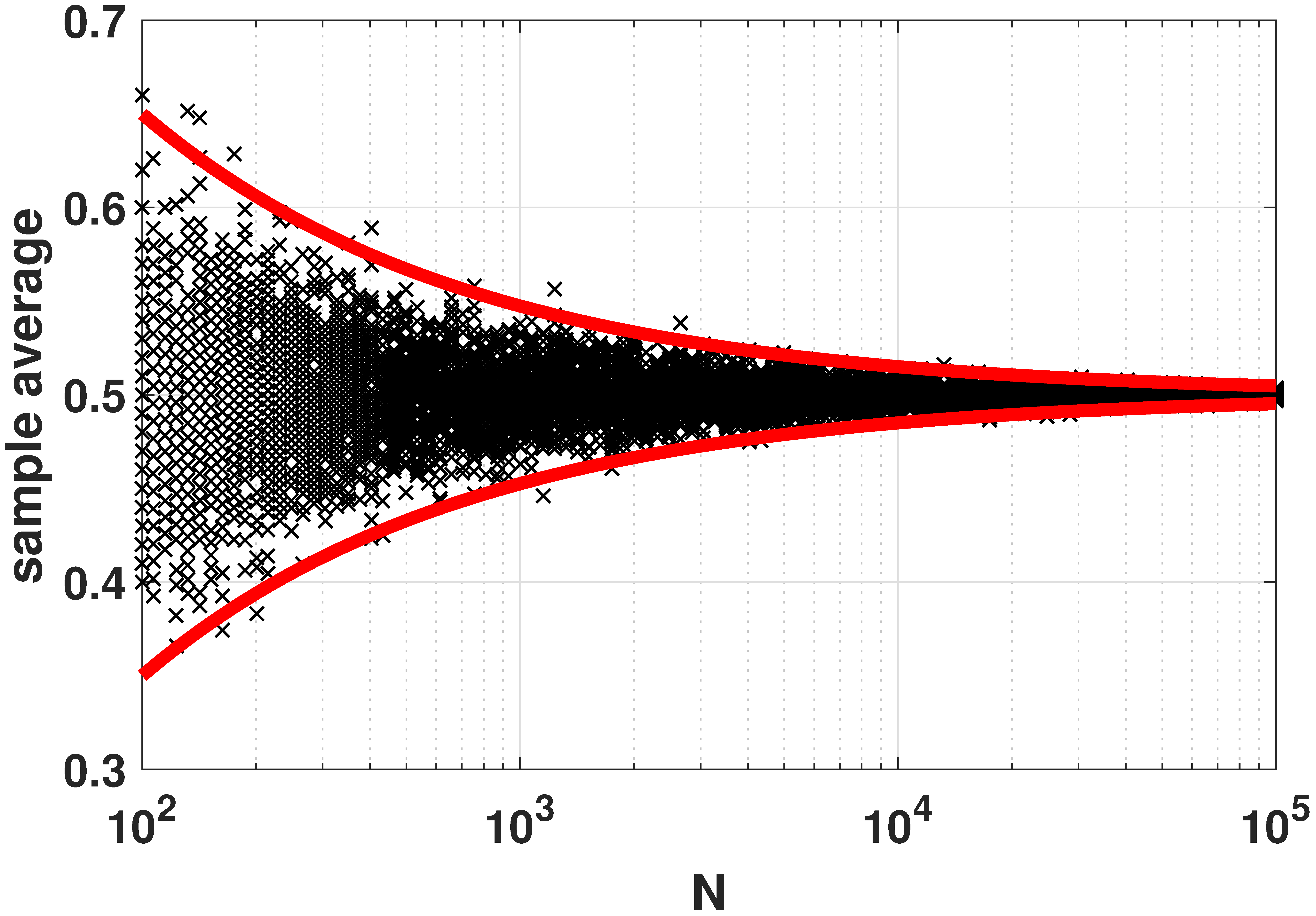
% MATLAB code to illustrate the weak law of large numbers
Nset = round(logspace(2,5,100));
for i=1:length(Nset)
    N = Nset(i);
    p = 0.5;
    x(:,i) = binornd(N, p, 1000,1)/N;
end
y = x(1:10:end,:)';
semilogx(Nset, y, 'kx'); hold on;
semilogx(Nset, p+3*sqrt(p*(1-p)./Nset), 'r', 'LineWidth', 4);
semilogx(Nset, p-3*sqrt(p*(1-p)./Nset), 'r', 'LineWidth', 4);

# Python code to illustrate the weak law of large numbers
import numpy as np
import matplotlib.pyplot as plt
import scipy.stats as stats
import numpy.matlib
p = 0.5
Nset = np.round(np.logspace(2,5,100)).astype(int)
x = np.zeros((1000,Nset.size))
for i in range(Nset.size):
  N = Nset[i]
  x[:,i] = stats.binom.rvs(N, p, size=1000)/N
Nset_grid = np.matlib.repmat(Nset, 1000, 1)
plt.semilogx(Nset_grid, x,'ko');
plt.semilogx(Nset, p + 3*np.sqrt((p*(1-p))/Nset), 'r', linewidth=6)
plt.semilogx(Nset, p - 3*np.sqrt((p*(1-p))/Nset), 'r', linewidth=6)

# Julia code to illustrate the weak law of large numbers
using Distributions, Plots

p = 0.5
Nset = round.((10).^range(2,5,length=100))
x = zeros(length(Nset), 1000)
for (i,N) in enumerate(Nset)
    x[i,:] = rand(Binomial(N, p), 1000) / N
end
y = x[:, 1:10:end]
scatter(Nset, y; xaxis=:log10, xticks=[1e2, 1e3, 1e4, 1e5],
        markershape=:x, color=:black,
        ylabel="sample average",
        legend=false)
plot!(Nset, p .+ 3*sqrt.(p*(1-p) ./ Nset); color=:red, linewidth=4)
plot!(Nset, p .- 3*sqrt.(p*(1-p) ./ Nset); color=:red, linewidth=4)

# R code to illustrate the weak law of large numbers

library(pracma)

p <- 0.5
Nset <- as.integer(round(logspace(2,5,100)))
x <- matrix(rep(0, 1000*length(Nset)), nrow=1000)
for (i in 1:length(Nset)) {
  N = Nset[i]
  x[,i] <- rbinom(1000, N, p) / N
}
Nset_grid <- repmat(Nset, m=1, n=1000)

semilogx(Nset_grid, x, col='black', pch=19)
points(Nset, p + 3*(((p*(1-p))/Nset)^(1/2)), col='red', pch=19, lwd=1)
points(Nset, p - 3*(((p*(1-p))/Nset)^(1/2)), col='red', pch=19, lwd=1)

% MATLAB: Plot the PDF of the sum of two Gaussians
figure;
n = 10000;
K = 2;
Z = zeros(1,n);
for i=1:K
    X = randi(6,1,n);
    Z = Z + X;
end
m = 3.5*K;
v = sqrt(K*(6^2-1)/12);
histogram(Z,K-0.5:6*K+0.5,'Normalization',...
    'probability','FaceColor',[0 0.5 0.8],'LineWidth',2);
set(gcf, 'Position', [100, 100, 600, 400]);
set(gca,'FontWeight','bold','fontsize',14);

# Julia: Plot the PDF of the sum of two Gaussians
using Distributions, Plots

n = 10000;
K = 2 # 6
X = DiscreteUniform(1, 6)
mu = mean(X)   # 3.5
sigma = std(X)    # sqrt((6^2-1)/12)
Z = sum(rand(X, n) for _ in 1:K)
mk = K * mu
sk = sqrt(K) * sigma
bin_range = (floor(mk - 3sk) - 1/2):(ceil(mk + 3sk) + 1/2)
plot_args = (normalize=true, color=RGB(0, 0.5, 0.8), linewidth=2, legend=false,
             bins=bin_range)

histogram(Z; plot_args..., title="⚁"^K)

# R: Plot the PDF of the sum of two Gaussians

library(pracma)

n <- 10000
K <- 2
Z <- rep(0, n)

for (i in 1:K) {
  X <- runif(n, min=1, max=6)
  Z <- Z + X
}
hist(Z,breaks=(K-0.5):(6*K+0.5),freq=FALSE)

% MATLAB: Visualize convergence in distribution
N = 10; % N = 50;
x = linspace(0,N,1001);
p = 0.5;
p_b = binopdf(x, N, p);
p_n = normpdf(x, N*p, sqrt(N*p*(1-p)));

c_b = binocdf(x, N, p);
c_n = normcdf(x, N*p, sqrt(N*p*(1-p)));

figure;
plot(x,p_b,'LineWidth',2,'Color',[0,0,0]); hold on;
plot(x,p_n,'LineWidth',6,'Color',[0.8,0,0]); hold off;
legend('Binomial', 'Gaussian', 'Location', 'Best');
grid on;
set(gcf, 'Position', [100, 100, 600, 400]);
set(gca,'FontWeight','bold','fontsize',14);

# Julia: Visualize convergence in distribution
using Distributions, Plots
N, p = 10, 0.5

B = Binomial(N,p)
Z = Normal(mean(B), std(B)) # N*p, sqrt(N*p*(1-p))

p_b(x) = pdf(B, x)
p_n(x) = pdf(Z, x)

c_b(x) = cdf(B, x)
c_n(x) = cdf(Z, x)

bin_args = (color = RGB(0, 0, 0), linewidth=2, label="Binomial")
norm_args = (color = RGB(0.8, 0, 0), linewidth=6, label="Normal")

ns = 0:N
p1 = plot(ns, p_b.(ns); bin_args..., seriestype=:sticks)
plot!(p_n, 0, N; norm_args...)

p2 = plot(c_b, 0, N; bin_args...)
plot!(c_n; norm_args...)

l = @layout [a b]
plot(p1, p2, layout=l)

# R: Visualize convergence in distribution

library(pracma)

N <- 10
N <- 50
x <- linspace(0, N, 1001)
p <- 0.5
p_b <- dbinom(x, N, p)
p_n <- dnorm(x, N*p, (N*p*(1-p))**(1/2))

c_b <- pbinom(x, N, p)
c_n <- pnorm(x, N*p, (N*p*(1-p))**(1/2))

plot(x, p_n, lwd=1, col='red')
lines(x, p_b, lwd=2, col='black')
legend("topright", c('Binomial', 'Gaussian'), fill=c('black', 'red'))

% MATLAB: Poisson to Gaussian: convergence in distribution
N = 4; % N = 10; % N = 50;
x = linspace(0,2*N,1001);
lambda = 1;
p_b = poisspdf(x, N*lambda);
p_n = normpdf(x, N*lambda, sqrt(N*lambda));

c_b = poisscdf(x, N*lambda);
c_n = normcdf(x, N*lambda, sqrt(N*lambda));

figure;
plot(x,p_b,'LineWidth',2,'Color',[0,0,0]); hold on;
plot(x,p_n,'LineWidth',6,'Color',[0.8,0,0]); hold off;
legend('Poisson', 'Gaussian', 'Location', 'NE');
grid on;
set(gcf, 'Position', [100, 100, 600, 400]);
set(gca,'FontWeight','bold','fontsize',18);

figure;
plot(x,c_b,'LineWidth',2,'Color',[0,0,0]); hold on;
plot(x,c_n,'LineWidth',6,'Color',[0.8,0,0]); hold off;
legend('Poisson', 'Gaussian', 'Location', 'SE');
grid on;
set(gcf, 'Position', [100, 100, 600, 400]);
set(gca,'FontWeight','bold','fontsize',18);

# Julia: Poisson to Gaussian: convergence in distribution
using Distributions, Plots

N = 4; # N = 10, N = 50;
lambda = 1

P = Poisson(N*lambda)
Z = Normal(mean(P), std(P))  # Nlambda, sqrt(Nlambda)

p_b(x) = pdf(P, x) # evaluate on integers
p_n(x) = pdf(Z, x)

c_b(x) = cdf(P, x)
c_n(x) = cdf(Z, x)

bin_args = (linewidth=2, color=RGB(0.0, 0.0, 0.0), label="Poisson")
norm_args = (linewidth=6, colr=RGB(0.8, 0.0, 0.0), label="Gaussian")

ns = 0:2N
p1 = plot(ns, p_b.(ns); bin_args..., seriestype=:sticks, legend=:topright)
plot!(p_n, 0, 2N; norm_args...)

p2 = plot(c_b, 0, 2N; bin_args..., legend=:bottomright)
plot!(c_n; norm_args...)

l = @layout [a b]
plot(p1, p2, layout=l)

# R: Poisson to Gaussian: convergence in distribution

library(pracma)

N <- 4
# N = 10
# N = 50

x <- linspace(0,2*N,1001)
lambda <- 1
p_b <- dpois(x, N*lambda)
p_n <- dnorm(x, N*lambda, sqrt(N*lambda))

c_b <- ppois(x, N*lambda);
c_n = pnorm(x, N*lambda, sqrt(N*lambda));

plot(x, p_n, col="red")
lines(x, p_b, col="black")
legend("topright", c('Poisson', 'Gaussian'), fill=c('black', 'red'))

plot(x, c_n, col="red")
lines(x, c_b, col="black")
legend("topright", c('Poisson', 'Gaussian'), fill=c('black', 'red'))

% MATLAB: Visualize the Central Limit Theorem
N = 10;
x = linspace(0,N,1001);
p = 0.5;
p_b = binopdf(x, N, p);
p_n = normpdf(x, N*p, sqrt(N*p*(1-p)));

c_b = binocdf(x, N, p);
c_n = normcdf(x, N*p, sqrt(N*p*(1-p)));

x2 = linspace(5-2.5,5+2.5,1001);
q2 = normpdf(x2,N*p, sqrt(N*p*(1-p)));

figure;
area(x2,q2,'EdgeColor','none','FaceColor',[0.6,0.9,1]); hold on;
plot(x,p_b,'LineWidth',2,'Color',[0,0,0]);
grid on;
set(gcf, 'Position', [100, 100, 600, 400]);
set(gca,'FontWeight','bold','fontsize',14);

figure;
area(x2,q2,'EdgeColor','none','FaceColor',[0.6,0.9,1]); hold on;
plot(x,p_n,'LineWidth',6,'Color',[0.8,0,0]);
grid on;
set(gcf, 'Position', [100, 100, 600, 400]);
set(gca,'FontWeight','bold','fontsize',14);

# Julia: Visualize the Central Limit Theorem
using Distributions, Plots

N = 10
x = range(0, N, length=1001)
p = 0.5


B = Binomial(N,p)
Z = Normal(mean(B), std(B))  # N*p, sqrt(N*p*(1-p))

p_b(x) = pdf(B, x)
p_n(x) = pdf(Z, x)

c_b(x) = cdf(B, x)
c_n(x) = cdf(Z, x)


xs = range(5-2.5, 5 + 2.5, length=1001)

p1 = plot(p_n, 5-2.5, 5+2.5; fillrange=0 .* xs, color=RGB(0.6, 0.9, 1.0), legend=false,
     title="Binomial PDF")
plot!(0:N, p_b.(0:N); color=RGB(0,0,0), linewidth=2, seriestype=:sticks, layout=1)


p2 = plot(p_n, 5-2.5, 5+2.5, fillrange=0 .* xs, color=RGB(0.6, 0.9, 1.0), legend=false,
     title = "Gaussian PDF")
plot!(p_n, 0, N; color=RGB(0.8, 0, 0), linewidth=6, layout=2)

l = @layout [a b]
plot(p1, p2, layout=l)

# R: Visualize the Central Limit Theorem

library(pracma)

N <- 10
x <- linspace(0,N,1001)
p <- 0.5
p_b <- dbinom(x, N, p);
p_n <- dnorm(x, N*p, sqrt(N*p*(1-p)));

c_b <- pbinom(x, N, p);
c_n <- pnorm(x, N*p, sqrt(N*p*(1-p)));

x2 <- linspace(5-2.5,5+2.5,1001);
q2 <- dnorm(x2,N*p, sqrt(N*p*(1-p)));

plot(x, p_n, col="red")
points(x, p_b, col="black", pch=19)

polygon(c(min(x2), x2, max(x2)), c(0, q2, 0), col='lightblue')

% MATLAB: Central Limit Theorem from moment generating functions
p = 0.5;
s = linspace(-10,10,1001);
MX = 1-p+p*exp(s);
N = 2;
semilogy(s, (1-p+p*exp(s/N)).^N, 'LineWidth',8, 'Color',[0.1,0.6,1]); hold on;
mu = p;
sigma = sqrt(p*(1-p)/N);
MZ = exp(mu*s + sigma^2*s.^2/2);
semilogy(s, MZ,':','LineWidth', 8, 'Color',[0,0,0]);
grid on;
axis([-10, 10 1e-2 1e5]);
legend('Binomial MGF', 'Gaussian MGF','Location','NW');
yticks([1e-2 1e-1 1 1e1 1e2 1e3 1e4 1e5]);
set(gcf, 'Position', [100, 100, 600, 400]);
set(gca,'FontWeight','bold','fontsize',24);

# Julia: Central Limit Theorem from moment generating functions
using Distributions, Plots

N = 2
p = 0.5;

B = Bernoulli(p)
mu, sigma = mean(B), std(B)/sqrt(N) # for Xbar
Z = Normal(mu, sigma)

m_Bernoulli(s) = mgf(B,s)    # (1 - p + p*exp(s))
m_B(s) = m_Bernoulli(s/N)^N  # (X1 + X2 + ... XN)/N
m_Z(s) = mgf(Z,s)            # exp(mu * s + sigma^2*s^2/2)

bin_args = (linewidth=8, color=RGB(0.1, 0.6, 1),
            yaxis=:log, yticks = [10.0^i for i in -1:4],
            label="Binomial MGF")
norm_args = (linewidth=8, color=RGB(0, 0, 0), yaxis=:log, linestyle=:dot, label="Gaussian MGF")

plot(m_B, -10, 10; bin_args..., legend=:topleft)
plot!(m_Z; norm_args...)

# R: How moment generating of Gaussian approximates in CLT

library(pracma)

p <- 0.5
s <- linspace(-10,10,1001)
MX <- 1-p+p*exp(s)
N <- 2
semilogy(s, (1-p+p*exp(s/N))**N, lwd=4, col="lightblue", xlim=c(-10,10), ylim=c(10**-2, 10**5))
mu <- p
sigma <- sqrt(p*(1-p)/N);
MZ <- exp(mu*s + sigma^2*s**2/2);
lines(s, MZ, lwd=4);
legend("topleft", c('Binomial MGF', 'Gaussian MGF'), fill=c('lightblue', 'black'))

% MATLAB: Failure of Central Limit Theorem at tails
x = linspace(-1,5,1001);
lambda = 1;

N = 1;
f1 = (sqrt(N)/lambda)*pdf('gamma',(x+sqrt(N))/(lambda/sqrt(N)),N,lambda);
semilogy(x, f1, 'LineWidth', 4, 'Color', [0.8 0.8 0.8]); hold on;

N = 10;
f2 = (sqrt(N)/lambda)*pdf('gamma',(x+sqrt(N))/(lambda/sqrt(N)),N,lambda);
semilogy(x, f2, 'LineWidth', 4, 'Color', [0.6 0.6 0.6]);

N = 100;
f3 = (sqrt(N)/lambda)*pdf('gamma',(x+sqrt(N))/(lambda/sqrt(N)),N,lambda);
semilogy(x, f3, 'LineWidth', 4, 'Color', [0.4 0.4 0.4]);

N = 1000;
f4 = (sqrt(N)/lambda)*pdf('gamma',(x+sqrt(N))/(lambda/sqrt(N)),N,lambda);
semilogy(x, f4, 'LineWidth', 4, 'Color', [0.2 0.2 0.2]);

g = pdf('norm',x,0,1);
semilogy(x, g, '-.', 'LineWidth', 4, 'Color', [0.9 0.0 0.0]);

grid on;
legend('N = 1', 'N = 10', 'N = 100', 'N = 1000', 'Gaussian', 'Location','SW');
axis([-1 5 min(ylim) max(ylim)]);
set(gcf, 'Position', [100, 100, 600, 400]);
set(gca,'FontWeight','bold','fontsize',18);

# Julia: Failure of Central Limit Theorem at tails
using Distributions, Plots


lambda = 1;

function gamma_pdf(N)
    function(x) # return anonymous function; also x -> ... notation
        (sqrt(N)/lambda) * pdf(Gamma(N,lambda), (x+sqrt(N))/(lambda/sqrt(N)))
    end
end
gaussian_pdf(x) = pdf(Normal(), x)


plot(gamma_pdf(1), -1, 5; linewidth=4, color=RGB(0.8, 0.8, 0.8), label="N=1",
     yaxis=:log,
     legend=:bottomleft)
plot!(gamma_pdf(10);   linewidth=4, color=RGB(0.6, 0.6, 0.6), label="N=10")
plot!(gamma_pdf(100);  linewidth=4, color=RGB(0.4, 0.4, 0.4), label="N=100")
plot!(gamma_pdf(1000); linewidth=4, color=RGB(0.2, 0.2, 0.2), label="N=1000")
plot!(gaussian_pdf;    linewidth=4, color=RGB(0.9, 0.0, 0.0), label="Gaussian",
      linestyle=:dash)

# R: Failure of Central Limit Theorem at tails

library(pracma)

x <- linspace(-1,5,1001)
lambda <- 1

N <- 1
f1 <- (N**(1/2)/lambda)*dgamma((x+sqrt(N))/(lambda/sqrt(N)), N, lambda)
semilogy(x, f1, lwd=1, col='lightgray', xlim=c(-1,5), ylim=c(10**-6, 1))

N <- 10
f1 <- (N**(1/2)/lambda)*dgamma((x+sqrt(N))/(lambda/sqrt(N)), N, lambda)
lines(x, f1, lwd=2, col='gray')

N <- 100
f1 <- (N**(1/2)/lambda)*dgamma((x+sqrt(N))/(lambda/sqrt(N)), N, lambda)
lines(x, f1, lwd=2, col='darkgray')

N <- 1000
f1 <- (N**(1/2)/lambda)*dgamma((x+sqrt(N))/(lambda/sqrt(N)), N, lambda)
lines(x, f1, lwd=2, col='black')

g <- dnorm(x,0,1)
lines(x, g, lwd=2, pch=1, col='red')

legend("bottomleft", c('N=1', 'N=10', 'N=100', 'N=1000', 'Gaussian'), fill=c('lightgray', 'gray', 'darkgray', 'black', 'red'))