eBook › Chapter 1 · Mathematical Background

Section 1.1

Infinite Series

Imagine that you have a fair coin. If you get a tail, you flip it again. You do this repeatedly until you finally get a head. What is the probability that you need to flip the coin three times to get one head?

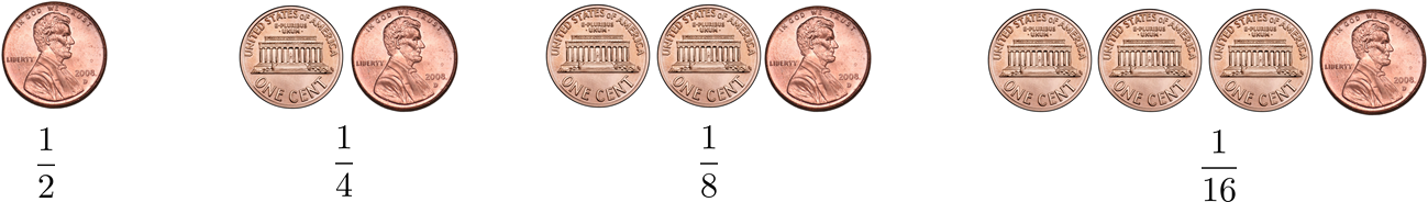
This is a warm-up exercise. Since the coin is fair, the probability of obtaining a head is $\frac{1}{2}$. The probability of getting a tail followed by a head is $\frac{1}{2} \times \frac{1}{2} = \frac{1}{4}$. Similarly, the probability of getting two tails and then a head is $\frac{1}{2} \times \frac{1}{2} \times \frac{1}{2} = \frac{1}{8}$. If you follow this logic, you can write down the probabilities for all other cases. For your convenience, we have drawn the first few in Figure 1.1. As you have probably noticed, the probabilities follow the pattern $\{\frac{1}{2},\frac{1}{4},\frac{1}{8},\ldots\}$.

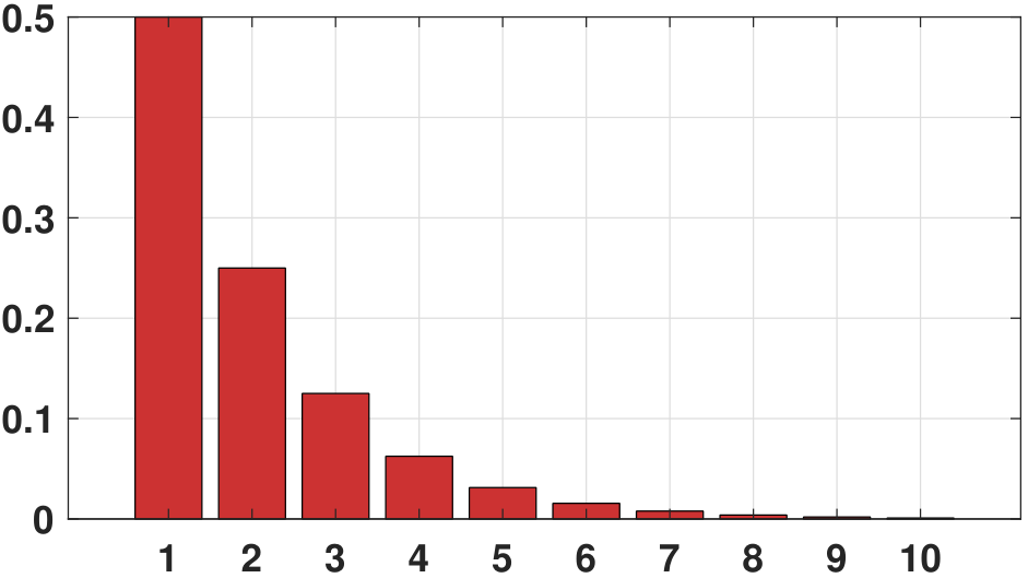
**Figure 1.1.** Suppose you flip a coin until you see a head. This requires you to have $N-1$ tails followed by a head. The probability of this sequence of events is $\frac{1}{2}$, $\frac{1}{4}$, $\frac{1}{8}$, …, which forms an infinite sequence.

We can also summarize these probabilities using a familiar plot called the histogram as shown in Figure 1.2. The histogram for this problem has a special pattern: each bar is half the height of the preceding one, and the sequence of bars extends infinitely.

Let us ask something harder: On average, if you want to be 90% sure that you will get a head, what is the minimum number of attempts you need to try? Five attempts? Ten attempts? Indeed, if you try ten attempts, you will very likely accomplish your goal. However, this would seem to be overkill. If you try five attempts, then it becomes unclear whether you will be 90% sure.

This problem can be answered by analyzing the sequence of probabilities. If we make two attempts, then the probability of getting a head is the sum of the probabilities for one attempt and that of two attempts:

\begin{aligned} \Pb[\text{success after 1 attempt}] &= \frac{1}{2} = 0.5\\ \Pb[\text{success after 2 attempts}] &= \frac{1}{2} + \frac{1}{4} = 0.75 \end{aligned}

Therefore, if you make 3 attempts or 4 attempts, you get the following probabilities:

\begin{aligned} \Pb[\text{success after 3 attempts}] &= \frac{1}{2} + \frac{1}{4} + \frac{1}{8} = 0.875\\ \Pb[\text{success after 4 attempts}] &= \frac{1}{2} + \frac{1}{4} + \frac{1}{8} + \frac{1}{16} = 0.9375. \end{aligned}

So if we try four attempts, we will have a 93.75% probability of getting a head. Thus, four attempts is the answer.

The MATLAB / Python codes we used to generate Figure 1.2 are shown below.

MATLAB

% MATLAB code to generate a geometric sequence
    p = 1/2;
    n = 1:10;
    X = p.^n;
    bar(n,X,'FaceColor',[0.8, 0.2,0.2]);

Python

# Python code to generate a geometric sequence
    import numpy as np
    import matplotlib.pyplot as plt
    p = 1/2
    n = np.arange(1,10)
    X = np.power(p,n)
    plt.bar(n,X); plt.show()

This warm-up exercise has perhaps raised some of your interest in the subject. However, we will not tell you everything now. We will come back to this in Chapter 3 when we discuss geometric random variables. In the present section, we want to make sure you have the basic mathematical tools to calculate quantities, such as a sum of fractional numbers. For example, what if we want to calculate $\Pb[\text{success after 107 attempts}]$? Is there a systematic way of performing the calculation?

Remark. You should be aware that the 93.75% only says that the probability of achieving the goal is high. If you have a bad day, you may still need more than four attempts. Therefore, when we stated the question, we asked for 90% “on average”. Sometimes you may need more attempts and sometimes fewer, but you have a 93.75% probability of success.

1.1.1Geometric Series

A geometric series is the sum of a finite or an infinite sequence of numbers with a constant ratio between successive terms. As we have seen in the previous example, a geometric series appears naturally in the context of discrete events. In Chapter 3 of this book, we will use geometric series when calculating the expectation and moments of a random variable.

Definition 1.1

Let $0 < r < 1$. A finite geometric sequence of power $n$ is a sequence of numbers $$\bigg\{1,r,r^2,\ldots,r^n\bigg\}.$$ An infinite geometric sequence is a sequence of numbers $$\bigg\{1,r,r^2,r^3,\ldots\bigg\}.$$

Theorem 1.1

The sum of a finite geometric series of power $n$ is

\sum_{k=0}^{n}r^k = 1+r+r^2+ \cdots+r^{n} = \frac{1-r^{n+1}}{1-r}.

Proof. We multiply both sides by $1-r$. The left-hand side becomes

\begin{aligned} \left(\sum_{k=0}^{n}r^k\right)\textcolor{blue}{(1-r)} &= \left(1+r+r^2+\cdots+r^n\right)\textcolor{blue}{(1-r)} \\ &= \left(1+r+r^2+\cdots+r^n \right)- \left(r+r^2+r^3+\cdots+r^{n+1}\right) \\ &\overset{(a)}{=} 1-r^{n+1}, \end{aligned}

where $(a)$ follows because consecutive terms cancel telescopically.

■

A corollary of Eq. (1.1) gives the sum of an infinite geometric series.

Corollary 1.1

Let $0 < r < 1$. The sum of an infinite geometric series is

\sum_{k=0}^{\infty}r^k = 1+r+r^2+ \cdots = \frac{1}{1-r}.

Proof. We take the limit in Eq. (1.1). This yields

\begin{aligned} \sum_{k=0}^{\infty}r^k &= \lim_{n\rightarrow \infty} \sum_{k=0}^{n}r^k = \lim_{n\rightarrow \infty} \frac{1-r^{n+1}}{1-r} = \frac{1}{1-r}. \end{aligned}

■

Remark. Note that the condition $0 < r < 1$ is important. If $r > 1$, then $r^{n+1} \to \infty$ as $n \to \infty$, so the series diverges. The constant $r$ cannot equal $1$, for otherwise the fraction $(1-r^{n+1})/(1-r)$ is undefined. We are not interested in the case when $r = 0$, because the sum is trivially 1: $\sum_{k=0}^{\infty} 0^k = 1 + 0^1 + 0^2 + \cdots = 1$.

Practice Exercise 1.1

Compute the infinite series $\sum\limits_{k=2}^\infty \frac{1}{2^k}$.

Solution

\begin{aligned} \sum_{k=2}^\infty \frac{1}{2^k} &= \frac{1}{4} + \frac{1}{8} + \cdots \\ &= \frac{1}{4} \left(1+ \frac{1}{2} + \frac{1}{4} + \cdots \right) \\ &= \frac{1}{4} \cdot \frac{1}{1-\frac{1}{2}} = \frac{1}{2}. \end{aligned}

Remark. You should not confuse a geometric series with a harmonic series. A harmonic series concerns the sum of $\{1,\frac{1}{2},\frac{1}{3},\frac{1}{4},\ldots\}$. It turns out that (This result can be found in Tom Apostol, Mathematical Analysis, 2nd Edition, Theorem 8.11.)

\sum_{n=1}^\infty \frac{1}{n} = 1 + \frac{1}{2} + \frac{1}{3} + \frac{1}{4} + \cdots = \infty.

On the other hand, a squared harmonic series $\{1,\frac{1}{2^2},\frac{1}{3^2},\frac{1}{4^2},\ldots\}$ converges:

\sum_{n=1}^\infty \frac{1}{n^2} = 1 + \frac{1}{2^2} + \frac{1}{3^2} + \frac{1}{4^2} + \cdots = \frac{\pi^2}{6}.

The latter result is known as the Basel problem.

We can extend the main theorem by considering more complicated series, for example, the following.

Corollary 1.2

Let $0 < r < 1$. It holds that

\sum_{k=1}^{\infty} k r^{k-1} = 1+2r+3r^2+ \cdots = \frac{1}{(1-r)^2}.

Proof. Take the derivative of both sides of Eq. (1.2). The left-hand side becomes

\begin{aligned} \frac{d}{dr} \sum_{k=0}^{\infty}r^k &= \frac{d}{dr} \left(1+r+r^2+ \cdots\right) \\ &= 1 + 2r + 3r^2 + \cdots = \sum_{k=1}^{\infty} k r^{k-1} \end{aligned}

The right-hand side becomes $\displaystyle \frac{d}{dr} \left(\frac{1}{1-r}\right) = \frac{1}{(1-r)^2}$.

■

Practice Exercise 1.2

Compute the infinite sum $\sum_{k=1}^{\infty} k \cdot \frac{1}{3^k}$.

Solution

We can use the derivative result:

\begin{aligned} \sum_{k=1}^{\infty} k \cdot \frac{1}{3^k} &= 1\cdot\frac{1}{3} + 2\cdot \frac{1}{9} + 3\cdot \frac{1}{27} + \cdots \\ &= \frac{1}{3} \cdot \left( 1 + 2 \cdot \frac{1}{3} + 3 \cdot \frac{1}{9} + \cdots \right) = \frac{1}{3} \cdot \frac{1}{(1-\frac{1}{3})^2} = \frac{1}{3}\cdot \frac{1}{\frac{4}{9}} = \frac{3}{4}. \end{aligned}

1.1.2Binomial Series

A geometric series is useful when handling situations such as $N-1$ failures followed by a success. However, we can easily twist the problem by asking: What is the probability of getting one head out of 3 independent coin tosses? In this case, the probability can be determined by enumerating all possible cases:

\begin{aligned} \Pb[\text{1 head in 3 coins}] &= \Pb[\text{H,T,T}] + \Pb[\text{T,H,T}] + \Pb[\text{T,T,H}] \\ &= \left(\frac{1}{2}\times\frac{1}{2}\times\frac{1}{2}\right) + \left(\frac{1}{2}\times\frac{1}{2}\times\frac{1}{2}\right) + \left(\frac{1}{2}\times\frac{1}{2}\times\frac{1}{2}\right)\\ &= \frac{3}{8}. \end{aligned}

Figure 1.3 illustrates the situation.

What lessons have we learned in this example? Notice that you need to enumerate all possible combinations of one head and two tails to solve this problem. The number is 3 in our example. In general, the number of combinations can be systematically studied using combinatorics, which we will discuss later in the chapter. However, the number of combinations motivates us to discuss another background technique known as the binomial series. The binomial series is instrumental in algebra when handling polynomials such as $(a+b)^2$ or $(1+x)^3$. It provides a valuable formula when computing these powers.

Theorem 1.2 (Binomial theorem)

For any real numbers $a$ and $b$ and any non-negative integer $n$, the binomial expansion of power $n$ is

(a+b)^n = \sum_{k=0}^n {n \choose k} a^{n-k}b^k,

where ${n \choose k} = \frac{n!}{k!(n-k)!}$.

The binomial theorem is valid for any real numbers $a$ and $b$ and any non-negative integer $n$. The quantity ${n \choose k}$ reads as “$n$ choose $k$”. Its definition is $${n \choose k} \bydef \frac{n!}{k!(n-k)!},$$ where $n! = n(n-1)(n-2)\cdots 3 \cdot 2 \cdot 1$. We shall discuss the physical meaning of ${n \choose k}$ in Section sec: ch1 combination. But we can quickly plug in the “$n$ choose $k$” into the coin flipping example by letting $n = 3$ and $k = 1$:

\begin{aligned} \text{Number of combinations for 1 head and 2 tails} = {3 \choose 1} = \frac{3!}{1!2!} = 3. \end{aligned}

So you can see why we want you to spend your precious time learning about the binomial theorem. In MATLAB and Python, ${n \choose k}$ can be computed using the commands as follows.

MATLAB

% MATLAB code to compute (N choose K) and K!
    n = 10;
    k = 2;
    nchoosek(n,k)
    factorial(k)

Python

# Python code to compute (N choose K) and K!
    from scipy.special import comb, factorial
    n = 10
    k = 2
    comb(n, k)
    factorial(k)

The binomial theorem makes the most sense when we also learn about Pascal's identity.

Theorem 1.3 (Pascal's identity)

Let $n$ and $k$ be positive integers such that $k \le n$. Then,

{n \choose k} + {n \choose k-1} = {n+1 \choose k}.

Proof. We start by recalling the definition of ${n \choose k}$. This gives us

\begin{aligned} {n \choose k} + {n \choose k-1} &= \frac{n!}{k!(n-k)!} + \frac{n!}{(k-1)!(n-(k-1))!} \\ &= n! \left( \frac{1}{k!(n-k)!} + \frac{1}{(k-1)!(n-k+1)!} \right), \end{aligned}

where we factor out $n!$ to obtain the second equation. Next, we observe that

\begin{aligned} \frac{1}{k!(n-k)!} \times \textcolor{blue}{\frac{(n-k+1)}{(n-k+1)}} &= \frac{n-k+1}{k!(n-k+1)!}, \\ \frac{1}{(k-1)!(n-k+1)!} \times \textcolor{blue}{\frac{k}{k}} &= \frac{k}{k!(n-k+1)!}. \end{aligned}

Substituting into the previous equation we obtain

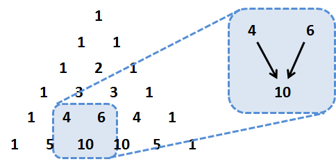
\begin{aligned} {n \choose k} + {n \choose k-1} &= n! \left(\frac{n-k+1}{k!(n-k+1)!} + \frac{k}{k!(n-k+1)!} \right) \\ &= n! \left(\frac{n+1}{k!(n-k+1)!}\right) \\ &= \frac{(n+1)!}{k!(n+1-k)!} = {n+1 \choose k}. \end{aligned}

■

Pascal's triangle is a visualization of the coefficients of $(a+b)^n$ as shown in Figure 1.4. For example, when $n = 5$, we know that ${5 \choose 3} = 10$. However, by Pascal's identity, we know that ${5 \choose 3} = {4 \choose 2} + {4 \choose 3}$. So the number 10 is actually obtained by summing the numbers 4 and 6 of the previous row.

Practice Exercise 1.3

Find $(1+x)^3$.

Solution

Using the binomial theorem, we can show that

\begin{aligned} (1+x)^3 &= \sum_{k=0}^3 {3 \choose k} 1^{3-k} x^k = 1 + 3x + 3x^2 + x^3. \end{aligned}

Practice Exercise 1.4

Let $0 < p <1$. Find $$\displaystyle\sum_{k=0}^n {n \choose k} p^{n-k}(1-p)^k.$$

Solution

By using the binomial theorem, we have

\begin{aligned} \sum_{k=0}^n {n \choose k} p^{n-k}(1-p)^k = (p + (1-p))^n = 1. \end{aligned}

This result will be helpful when evaluating binomial random variables in Chapter 3.

We now prove the binomial theorem. Please feel free to skip the proof if this is your first time reading the book.

Proof of the binomial theorem. We prove by induction. When $n = 1$,

\begin{aligned} (a+b)^1 &= a+b = \sum_{k=0}^1 a^{1-k}b^k. \end{aligned}

Therefore, the base case is verified. Assume up to case $n$. We need to verify case $n+1$.

\begin{aligned} (a+b)^{n+1} = (a+b)(a+b)^n &= (a+b) \sum_{k=0}^n {n \choose k} a^{n-k}b^k \\ &= \sum_{k=0}^n {n \choose k} a^{n-k+1}b^k + \sum_{k=0}^n {n \choose k} a^{n-k}b^{k+1}. \end{aligned}

We want to apply Pascal's identity to combine the two terms. In order to do so, we note that the second term in this sum can be rewritten as

\begin{aligned} \sum_{k=0}^n {n \choose k} a^{n-k}b^{k+1} &= \sum_{k=0}^n {n \choose k} a^{n+1-k-1}b^{k+1} \\ &= \sum_{\ell=1}^{n+1} {n \choose \ell-1} a^{n+1-\ell}b^{\ell}, \quad\quad \mbox{where} \quad \ell = k+1\\ &= \sum_{\ell=1}^{n} {n \choose \ell-1} a^{n+1-\ell}b^{\ell} + b^{n+1}. \end{aligned}

The first term in the sum can be written as

\begin{aligned} \sum_{k=0}^n {n \choose k} a^{n-k+1}b^k &= \sum_{\ell=1}^n {n \choose \ell} a^{n+1-\ell}b^\ell + a^{n+1}, \end{aligned}

where the $k=0$ term is separated as $a^{n+1}$. Therefore, the two terms can be combined using Pascal's identity to yield

\begin{aligned} (a+b)^{n+1} &= \sum_{\ell=1}^n \left[{n \choose \ell} + {n \choose \ell-1}\right] a^{n+1-\ell}b^\ell + a^{n+1} + b^{n+1}\\ &= \sum_{\ell=1}^n {n+1 \choose \ell} a^{n+1-\ell}b^\ell + a^{n+1} + b^{n+1} = \sum_{\ell=0}^{n+1} {n+1 \choose \ell} a^{n+1-\ell}b^\ell. \end{aligned}

Hence, the ($n+1$)th case is also verified. By the principle of mathematical induction, we have completed the proof.

■

The end of the proof. Please join us again.