eBook › Chapter 1 · Mathematical Background

Section 1.3

Integration

When you learned calculus, your teacher probably told you that there are two ways to compute an integral:

sep0ex
Substitution: $$\int f(ax) \; dx = \frac{1}{a}\int f(u) \; du.$$
By parts: $$\int u \; dv = u \, v - \int v \; du.$$

Besides these two, we want to teach you two more. The first technique is even and odd functions when integrating a function symmetrically about the $y$-axis. If a function is even, you just need to integrate half of the function. If a function is odd, you will get a zero. The second technique is to leverage the fact that a probability density function integrates to 1. We will discuss the first technique here and defer the second technique to Chapter 4.

Besides the two integration techniques, we will review the fundamental theorem of calculus. We will need it when we study cumulative distribution functions in Chapter 4.

1.3.1Odd and even functions

Definition 1.3

A function $f: \R \rightarrow \R$ is even if for any $x \in \R$,

$$f(x) = f(-x),$$

and $f$ is odd if

$$f(x) = -f(-x).$$

Essentially, an even function flips over about the $y$-axis, whereas an odd function flips over both the $x$- and $y$-axes.

Example 1.3

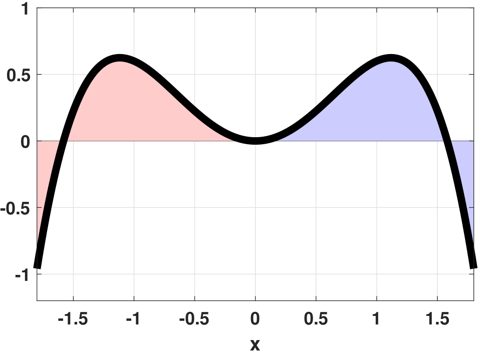
The function $f(x) = x^2 - 0.4x^4$ is even, because

$$f(-x) = (-x)^2 - 0.4(-x)^4 = x^2-0.4x^4 = f(x).$$

See Figure 1.9(a) for illustration. When integrating the function, we have

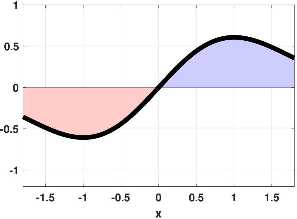
\begin{aligned} \int_{-1}^1 f(x) \; dx = 2\int_{0}^1 f(x) \; dx &= 2 \int_{0}^1 \left(x^2 - 0.4x^4\right) \; dx = 2 \bigg[\frac{x^3}{3}-\frac{0.4}{5}x^5\bigg]_{x=0}^{x=1} = \frac{38}{75}. \end{aligned}

Example 1.4

The function $f(x) = x\exp(-x^2/2)$ is odd, because

f(-x) = (-x)\exp\left\{-\frac{(-x)^2}{2}\right\} = -x\exp\left\{-\frac{x^2}{2}\right\} = -f(x).

See Figure 1.9(b) for illustration. When integrating the function, we can let $u = -x$. Then, the integral becomes

\begin{aligned} \int_{-1}^1 f(x) \; dx &= \int_{-1}^{0} f(x) \; dx + \int_{0}^{1} f(x) \; dx \\ &= \int_{0}^{1} f(-u) \; du + \int_{0}^{1} f(x) \; dx \\ &= -\int_{0}^{1} f(u) \; du + \int_{0}^{1} f(x) \; dx = 0. \end{aligned}

**Figure 1.9.** An even function is symmetric about the $y$-axis, and so the integration $\int_{-a}^a f(x) \; dx = 2\int_0^a f(x) \; dx$. An odd function is anti-symmetric about the $y$-axis. Thus, $\int_{-a}^a f(x) \; dx = 0$.

1.3.2Fundamental Theorem of Calculus

Our following result is the Fundamental Theorem of Calculus. It is a handy tool that links integration and differentiation.

Theorem 1.5 (Fundamental Theorem of Calculus)

Let $f: [a, b] \rightarrow \R$ be a continuous function defined on a closed interval $[a,b]$. Then, for any $x \in (a,b)$,

f(x) = \frac{d}{dx} \int_{a}^x f(t) \; dt,

Before we prove the result, let us understand the theorem if you have forgotten its meaning.

Example 1.5

Consider a function $f(t) = t^2$. If we integrate the function from $0$ to $x$, we will obtain another function

F(x) \bydef \int_{0}^{x} f(t) \; dt = \int_{0}^x t^2 \; dt = \frac{x^3}{3}.

On the other hand, we can differentiate $F(x)$ to obtain $f(x)$:

f(x) = \frac{d}{dx}F(x) = \frac{d}{dx} \frac{x^3}{3} = x^2.

The fundamental theorem of calculus basically puts the two together: $$f(x) = \frac{d}{dx}\int_{0}^x f(t) \; dt.$$ That's it. Nothing more and nothing less.

How can the fundamental theorem of calculus ever be useful when studying probability? Very soon you will learn two concepts: probability density function and cumulative distribution function. These two functions are related to each other by the fundamental theorem of calculus. To give you a concrete example, we write down the probability density function of an exponential random variable. (Please do not panic about the exponential random variable. Just think of it as a “rapidly decaying” function.)

f(x) = e^{-x}, \;\; x \ge 0.

It turns out that the cumulative distribution function is

\begin{aligned} F(x) = \int_{0}^{x} f(t) \; dt = \int_0^x e^{-t}\; dt = 1-e^{-x}. \end{aligned}

You can also check that $f(x) = \frac{d}{dx}F(x)$. The fundamental theorem of calculus says that if you tell me $F(x) = \int_0^x e^{-t}\; dt$ (for whatever reason), I will be able to tell you that $f(x) = e^{-x}$ merely by visually inspecting the integrand without doing the differentiation.

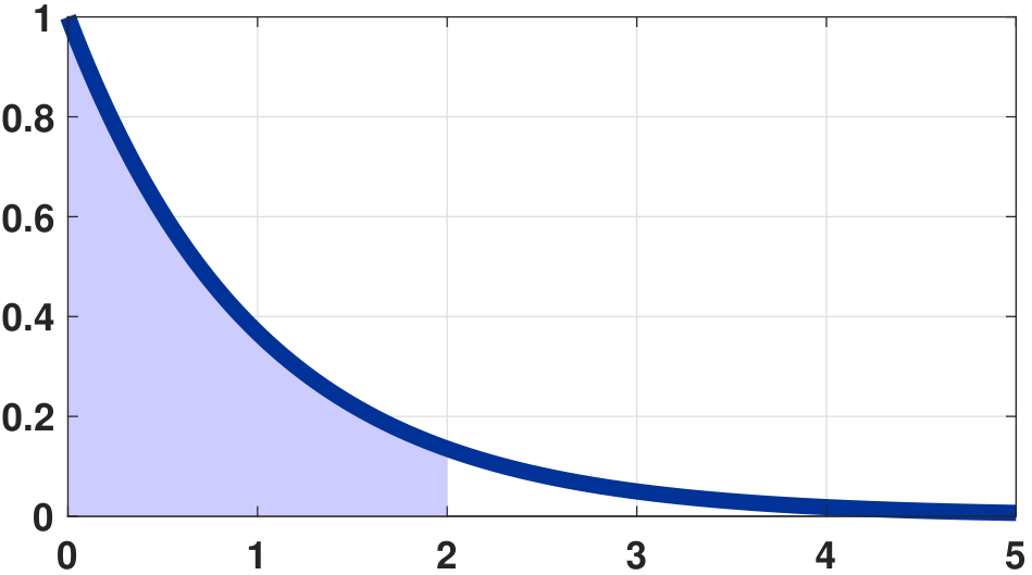
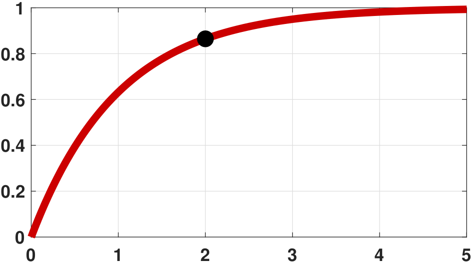
**Figure 1.10.** The pair of functions $f(x) = e^{-x}$ and $F(x) = 1-e^{-x}$

Figure 1.10 illustrates the pair of functions $f(x) = e^{-x}$ and $F(x) = 1-e^{-x}$. One thing you should notice is that the height of $F(x)$ is the area under the curve of $f(t)$ from $-\infty$ to $x$. For example, in Figure 1.10 we show the area under the curve from 0 to $2$. Correspondingly in $F(x)$, the height is $F(2)$.

The following proof of the Fundamental Theorem of Calculus can be skipped if it is your first time reading the book.

Proof. Our proof is based on Stewart (6th Edition), Section 5.3. Define the integral as a function $F$: $$F(x) = \int_{a}^x f(t) \; dt.$$ The derivative of $F$ with respect to $x$ is

\begin{aligned} \frac{d}{dx} F(x) &= \lim_{h \rightarrow 0} \frac{F(x+h) - F(x)}{h} \\ &= \lim_{h \rightarrow 0} \frac{1}{h} \left(\int_{a}^{x+h} f(t) \; dt - \int_{a}^{x} f(t) \; dt \right)\\ &= \lim_{h \rightarrow 0} \frac{1}{h} \int_{x}^{x+h} f(t) \; dt \\ &\overset{(a)}{\le} \lim_{h \rightarrow 0} \frac{1}{h} \int_{x}^{x+h} \left\{ \max_{ x \le \tau \le x+h} f(\tau) \right\} \; dt\\ &= \lim_{h \rightarrow 0} \left\{ \max_{ x \le \tau \le x+h} f(\tau) \right\}. \end{aligned}

Here, the inequality in $(a)$ holds because $$f(t) \le \max\limits_{ x \le \tau \le x+h} f(\tau)$$ for all $x \le t \le x+h$. The maximum exists because $f$ is continuous in a closed interval.

Using the parallel argument, we can show that

\begin{aligned} \frac{d}{dx} F(x) &= \lim_{h \rightarrow 0} \frac{F(x+h) - F(x)}{h} \\ &= \lim_{h \rightarrow 0} \frac{1}{h} \left(\int_{a}^{x+h} f(t) \; dt - \int_{a}^{x} f(t) \; dt \right)\\ &= \lim_{h \rightarrow 0} \frac{1}{h} \int_{x}^{x+h} f(t) \; dt\\ &\ge \lim_{h \rightarrow 0} \frac{1}{h} \int_{x}^{x+h} \left\{ \min_{ x \le \tau \le x+h} f(\tau) \right\} \; dt \\ &= \lim_{h \rightarrow 0} \left\{ \min_{ x \le \tau \le x+h} f(\tau) \right\}. \end{aligned}

Combining the two results, we have that

\lim_{h \rightarrow 0} \left\{ \min_{ x \le \tau \le x+h} f(\tau) \right\} \le \frac{d}{dx} F(x) \le \lim_{h \rightarrow 0} \left\{ \max_{ x \le \tau \le x+h} f(\tau) \right\}.

However, since the two limits are both converging to $f(x)$ as $h\rightarrow 0$, we conclude that $\frac{d}{dx} F(x) = f(x)$.

■

Remark. An alternative proof is to use the Mean Value Theorem in terms of Riemann-Stieltjes integrals (see, e.g., Tom Apostol, Mathematical Analysis, 2nd edition, Theorem 7.34). To handle general functions such as delta functions, one can use techniques in Lebesgue's integration. However, this is beyond the scope of this book.

This is the end of the proof. Please join us again.

In many practical problems, the fundamental theorem of calculus needs to be used in conjunction with the chain rule.

Corollary 1.3

Let $f: [a, b] \rightarrow \R$ be a continuous function defined on a closed interval $[a,b]$. Let $g: \R \rightarrow [a,b]$ be a continuously differentiable function. Then, for any $x \in (a,b)$,

\frac{d}{dx} \int_{a}^{g(x)} f(t) \; dt = g'(x) \cdot f(g(x)).

Proof. We can prove this with the chain rule: Let $y = g(x)$. Then we have

\begin{aligned} \frac{d}{dx} \int_{a}^{g(x)} f(t) \; dt = \frac{d y}{dx} \cdot \frac{d}{d y}\int_{a}^{y} f(t) \; dt = g'(x) \; f(y), \end{aligned}

which completes the proof.

■

Practice Exercise 1.6

Evaluate the integral

\frac{d}{d x} \int_{0}^{x-\mu} \frac{1}{\sqrt{2\pi \sigma^2}} \exp\left\{-\frac{t^2}{2\sigma^2}\right\} \; dt.

Solution

Let $y = x- \mu$. Then by using the fundamental theorem of calculus, we can show that

\begin{aligned} \frac{d}{d x} \int_{0}^{x-\mu} \frac{1}{\sqrt{2\pi \sigma^2}} \exp\left\{-\frac{t^2}{2\sigma^2}\right\} \; dt &= \frac{dy}{dx} \cdot \frac{d}{dy} \int_{0}^{y} \frac{1}{\sqrt{2\pi \sigma^2}} \exp\left\{-\frac{t^2}{2\sigma^2}\right\} \; dt \\ &= \frac{d (x-\mu)}{dx} \cdot \frac{1}{\sqrt{2\pi \sigma^2}} \exp\left\{-\frac{y^2}{2\sigma^2}\right\}\\ &= \frac{1}{\sqrt{2\pi \sigma^2}} \exp\left\{-\frac{(x-\mu)^2}{2\sigma^2}\right\}. \end{aligned}

This result will be useful when we do linear transformations of a Gaussian random variable in Chapter 4.