Maximum-Likelihood Estimation

Maximum-likelihood (ML) estimation, as the name suggests, is an estimation method that “maximizes” the “likelihood”. Therefore, to understand the ML estimation, we first need to understand the meaning of likelihood, and why maximizing the likelihood would be useful.

8.1.1Likelihood function

Consider a set of \(N\) data points \(\calD = \{x_1,x_2,\ldots,x_N\}\). We want to describe these data points using a probability distribution. What would be the most general way of defining such a distribution?

Since we have \(N\) data points, and we do not know anything about them, the most general way to define a distribution is as a high-dimensional probability density function (PDF) \(f_{\mX}(\vx)\). This is a PDF of a random vector \(\mX = [X_1,\ldots,X_N]^T\). A particular realization of this random vector is \(\vx = [x_1,\ldots,x_N]^T\).

\(f_{\mX}(\vx)\) is the most general description for the \(N\) data points because \(f_{\mX}(\vx)\) is the joint PDF of all variables. It provides the complete statistical description of the vector \(\mX\). For example, we can compute the mean vector \(\E[\mX]\), the covariance matrix \(\Cov(\mX)\), the marginal distributions, the conditional distribution, the conditional expectations, etc. In short, if we know \(f_{\mX}(\vx)\), we know everything about \(\mX\).

The joint PDF \(f_{\mX}(\vx)\) is always parameterized by a certain parameter \(\vtheta\). For example, if we assume that \(\mX\) is drawn from a joint Gaussian distribution, then \(f_{\mX}(\vx)\) is parameterized by the mean vector \(\vmu\) and the covariance matrix \(\mSigma\). So we say that the parameter \(\vtheta\) is \(\vtheta = (\vmu, \mSigma)\). To state the dependency on the parameter explicitly, we write

When you express the joint PDF as a function of \(\vx\) and \(\vtheta\), you have two variables to play with. The first variable is the observation \(\vx\), which is given by the measured data. We usually think about the probability density function \(f_{\mX}(\vx)\) in terms of \(\vx\), because the PDF is evaluated at \(\mX = \vx\). In estimation, however, \(\vx\) is something that you cannot control. When your boss hands a dataset to you, \(\vx\) is already fixed. You can consider the probability of getting this particular \(\vx\), but you cannot change \(\vx\).

The second variable stated in \(f_{\mX}(\vx; \, \vtheta)\) is the parameter \(\vtheta\). This parameter is what we want to find out, and it is the subject of interest in an estimation problem. Our goal is to find the optimal \(\vtheta\) that can offer the “best explanation” to data \(\vx\), in the sense that it can maximize \(f_{\mX}(\vx; \, \vtheta)\).

The likelihood function is the PDF that shifts the emphasis to \(\vtheta\):

A word of caution: \(\calL(\vtheta \,|\, \vx)\) is not a conditional PDF because \(\vtheta\) is not a random variable. The correct way to interpret \(\calL(\vtheta \,|\, \vx)\) is to view it as a function of \(\vtheta\). This function changes its shape according to the observed data \(\vx\). We will return to this point shortly.

Independent observations

While \(f_{\mX}(\vx)\) provides us with a complete picture of the \(\mX\), using \(f_{\mX}(\vx)\) is tedious. We need to describe how each \(X_n\) is generated and describe how \(X_n\) is related to \(X_m\) for all pairs of \(n\) and \(m\). If the vector \(\mX\) contains \(N\) entries, then there are \(N^2/2\) pairs of correlations we need to compute. When \(N\) is large, finding \(f_{\mX}(\vx)\) would be very difficult if not impossible.

In practice, \(f_{\mX}(\vx)\) may sometimes be overkill. For example, if we measure the inter-arrival time of a bus for several days, it is quite likely that the measurements will not be correlated. In this case, instead of using the full \(f_{\mX}(\vx)\), we can make assumptions about the data points. The assumption we will make is that all the data points are independent and that they are drawn from an identical distribution \(f_X(x)\). The assumption that the data points are independently and identically distributed (i.i.d.) significantly simplifies the problem so that the joint PDF \(f_{\mX}\) can be written as a product of single PDFs \(f_{X_n}\):

If you prefer a visualization, we can take a look at the covariance matrix, which goes from a full covariance matrix to a diagonal matrix and then to an identity matrix:

The assumption of i.i.d. is strong. Not all data can be modeled as i.i.d. (For example, photons passing through a scattering medium have correlated statistics.) However, if the i.i.d. assumption is valid, we can simplify the model significantly.

If the data points are i.i.d., then we can write the joint PDF as

This simplifies the likelihood function as a product of the individual PDFs.

In computation we often take the log of the likelihood function. We call the resulting function the log-likelihood.

Visualizing the likelihood function

The likelihood function \(\calL(\vtheta\,|\,\vx)\) is a function of \(\vtheta\), but its value also depends on the underlying measurements \(\vx\). It is extremely important to keep in mind the presence of both.

To help you visualize the effect of \(\vtheta\) and \(\vx\), we consider a set of i.i.d. Bernoulli random variables. As we have just shown in the practice exercise, the likelihood function of these i.i.d. random variables is

where we define \(S = \sum_{n=1}^N x_n\) as the sum of the (binary) measurements.

To make the dependency on \(S\) and \(\theta\) explicit, we write \(\calL(\theta\,|\vx)\) as

which emphasizes the role of \(S\) in defining the log-likelihood function. We plot the surface of \(L(\theta\,|\,S)\) as a function of \(S\) and \(\theta\), assuming that \(N = 50\). As shown on the left-hand side of Figure 8.1, the surface \(L(\theta|S)\) has a saddle shape. Along one direction the function goes up, whereas along another direction the function goes down. In the middle of Figure 8.1, we show a bird's-eye view of the surface, with the color-coding matched with the surface plot. As you can see, when plotted as a function of \(\theta\) and \(\vx\) (in our case, we use a summary statistic \(S = \sum_{n=1}^N x_n\)), the two-dimensional plot tells us how the log-likelihood function changes when \(S\) changes. On the right-hand side of Figure 8.1, we show two particular cross sections of the two-dimensional plot. One cross section is taken from \(S = 25\) and the other cross section is taken from \(S = 12\). Since the total number of heads in this numerical experiment is assumed to be \(N = 50\), the first cross section at \(S = 25\) is obtained when half of the Bernoulli measurements are “1”, whereas the second cross section at \(S = 12\) is obtained when a quarter of the Bernoulli measurements are “1”.

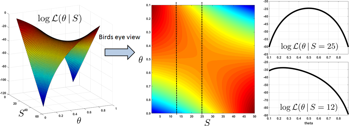
The cross sections tell us the log-likelihood function \(\log \calL(\theta|S)\) is a function defined specifically for a given measurement \(\vx\). As you can see from Figure 8.1, the log-likelihood function changes when \(S\) changes. Therefore, if our goal is to “find a \(\theta\) that maximizes the log-likelihood function”, then for a different \(\vx\) we will have a different answer. For example, according to Figure 8.1, the maximum for \(\log \calL(\theta|S = 25)\) occurs when \(\theta \approx 0.5\), and the maximum for \(\log \calL(\theta|S = 12)\) occurs when \(\theta \approx 0.24\). These are the maximum-likelihood estimates for the respective measurements.

We use the following MATLAB code to generate the surface plot:

% MATLAB code to generate the surface plot
    N = 50;
    S = 1:N;
    theta = linspace(0.1,0.9,100);
    [S_grid, theta_grid] = meshgrid(S, theta);
    L = S_grid.*log(theta_grid) + (N-S_grid).*log(1-theta_grid);
    s = surf(S,theta,L);
    s.LineStyle   = '-';
    colormap jet
    view(65,15)

For the bird's-eye view plot, we replace surf with imagesc(S,theta,L). For the cross section plots, we call the commands plot(theta, L(:,12)) and plot(theta, L(:,25)).

8.1.2Maximum-likelihood estimate

The likelihood is the PDF of \(\mX\) but viewed as a function of \(\vtheta\). The optimization problem of maximizing \(\calL(\vtheta\,|\,\vx)\) is called the maximum-likelihood (ML) estimation:

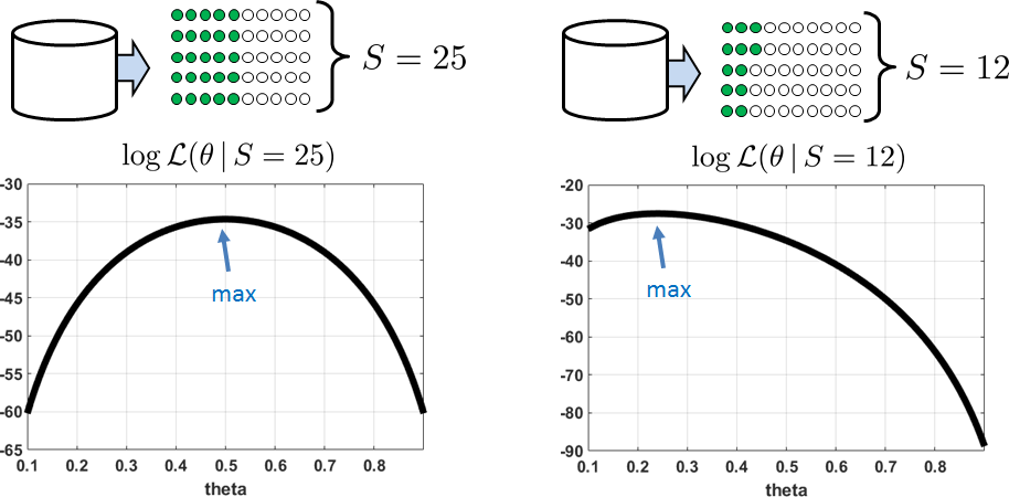
Let's do a sanity check to see if this result makes sense. The solution to this problem says that \(\thetahat_{\text{ML}}\) is the empirical average of the measurements. Assume that \(N = 50\). Let us consider two particular scenarios as illustrated in Figure 8.2.

• sep0ex
• Scenario 1: \(\vx\) is a vector of measurements such that \(S \bydef \sum_{n=1}^N x_n = 25\). Since \(N = 50\), the formula tells us that \(\thetahat_{\text{ML}} = \frac{25}{50} = 0.5\). This is the best guess based on the 50 measurements where 25 are heads. If you look at Figure 8.1 and Figure 8.2, when \(S = 25\), we are looking at a particular cross section in the 2D plot. The likelihood function we are inspecting is \(\calL(\theta|S=25)\). For this likelihood function, the maximum occurs at \(\theta = 0.5\).
• Scenario 2: \(\vx\) is a vector of measurements such that \(S \bydef \sum_{n=1}^N x_n = 12\). The formula tells us that \(\thetahat_{\text{ML}} = \frac{12}{50} = 0.24\). This is again the best guess based on the 50 measurements where 12 are heads. Referring to Figure 8.1 and Figure 8.2, we can see that the likelihood function corresponds to another cross section \(\calL(\theta|S=12)\) where the maximum occurs at \(\theta = 0.24\).

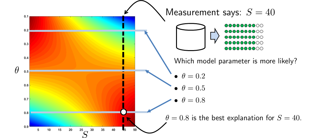
At this point, you may wonder why the shape of the likelihood function \(\calL(\theta\,|\,\vx)\) changes so radically as \(\vx\) changes? The answer can be found in Figure 8.3. Imagine that we have \(N = 50\) measurements of which \(S = 40\) give us heads. If these i.i.d. Bernoulli random variables have a parameter \(\theta = 0.5\), it is quite unlikely that we will get 40 out of 50 measurements to be heads. (If it were \(\theta = 0.5\), we should get more or less 25 out of 50 heads.) When \(S = 40\), and without any additional information about the experiment, the most logical guess is that the Bernoulli random variables have a parameter \(\theta = 0.8\). Since the measurement \(S\) can be as extreme as 0 out of 50 or 50 out of 50, the likelihood function \(\calL(\theta\,|\,\vx)\) has to reflect these extreme cases. Therefore, as we change \(\vx\), we observe a big change in the shape of the likelihood function.

As you can see from Figure 8.3, \(S = 40\) corresponds to the marked vertical cross section. As we determine the maximum-likelihood estimate, we search among all the possibilities, such as \(\theta = 0.2\), \(\theta = 0.5\), \(\theta = 0.8\), etc. These possibilities correspond to the horizontal lines we drew in the figure. Among those horizontal lines, it is clear that the best estimate occurs when \(\theta = 0.8\), which is also the ML estimate.

Visualizing ML estimation as \(N\) grows

Maximum-likelihood estimation can also be understood directly from the PDF instead of the likelihood function. To explain this perspective, let's do a quick exercise.

Now we will draw the PDF and compare it with the measured data points. Our focus is to analyze how the ML estimate changes as \(N\) grows.

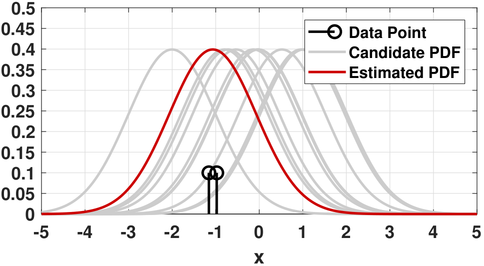
When \(N = 1\). There is only one observation \(x_1\). The best Gaussian that fits this sample must be the one that is centered at \(x_1\). In fact, the optimization is (We skip the step of checking whether the stationary point is a maximum or a minimum, which can be done by evaluating the second-order derivative. In fact, since the function \(-(x_1 - \theta)^2\) is concave in \(\theta\), a stationary point must be a maximum.)

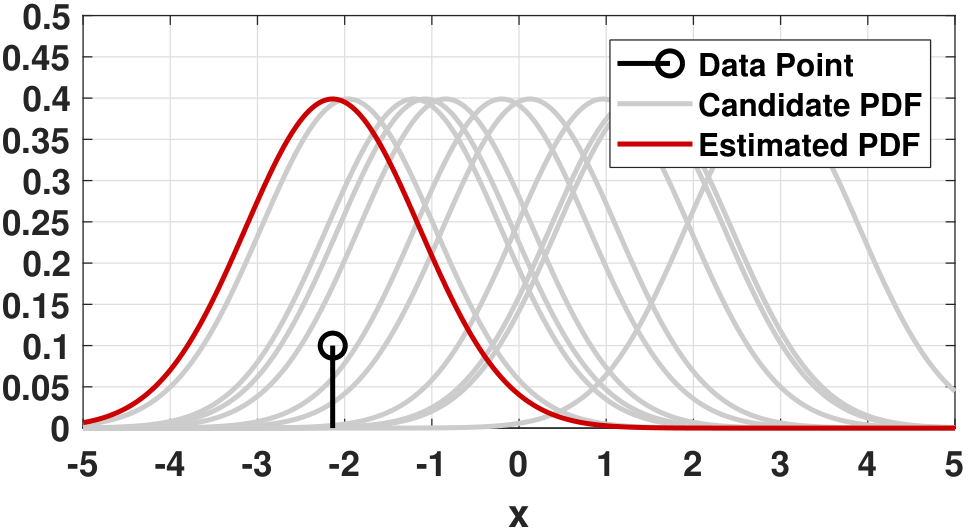
Therefore, the ML estimate is \(\widehat{\theta}_{\text{ML}} = x_1\). Figure 8.4 illustrates this case. As we conduct the ML estimation, we imagine that there are a few candidate PDFs. The ML estimation says that among all these candidate PDFs we need to find one that can maximize the probability of obtaining the observation \(x_1\). Since we only have one observation, we have no choice but to pick a Gaussian centered at \(x_1\). Certainly the sample \(X_1 = x_1\) could be bad, and we may find a wrong Gaussian. However, with only one sample there is no way for us to make better decisions.

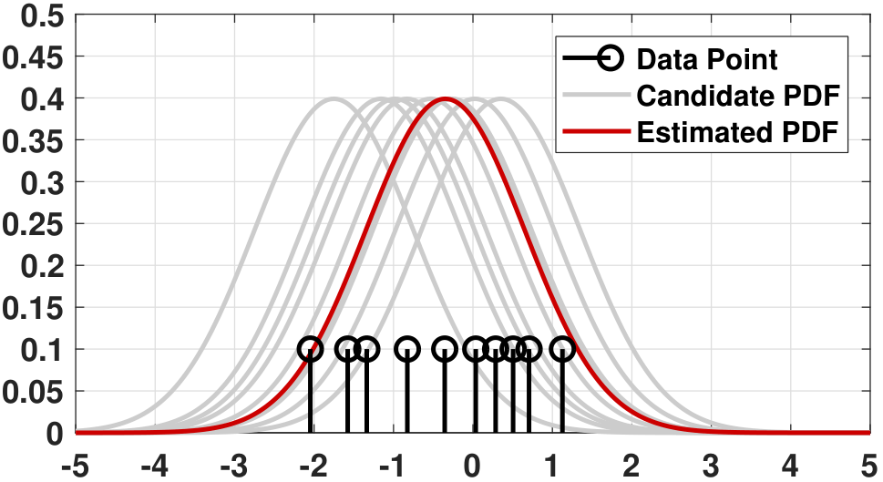
When \(N = 2\). In this case we need to find a Gaussian that fits both \(x_1\) and \(x_2\). The probability of simultaneously observing \(x_1\) and \(x_2\) is determined by the joint distribution. By independence we then have

where the last step is obtained by taking the derivative: $$\frac{d}{d\theta}\left\{ (x_1-\theta)^2 + (x_2-\theta)^2\right\} = 2(x_1-\theta) + 2(x_2-\theta).$$ Equating this with zero yields the solution \(\theta = \frac{x_1+x_2}{2}\). Therefore, the best Gaussian that fits the observations is \(\text{Gaussian}(\frac{x_1+x_2}{2},\sigma^2)\).

Does this result make sense? When you have two data points \(x_1\) and \(x_2\), the ML estimation is trying to find a Gaussian that can best fit both of these two data points. Your best bet here is \(\thetahat_{\text{ML}} = (x_1+x_2)/2\), because there are no other choices. If you choose \(\thetahat_{\text{ML}} = x_1\) or \(\thetahat_{\text{ML}} = x_2\), it cannot be a good estimate because you are not using both data points. As shown in Figure 8.5, for these two observed data points \(x_1\) and \(x_2\), the PDF marked in red (which is a Gaussian centered at \((x_1+x_2)/2\)) is indeed the best fit.

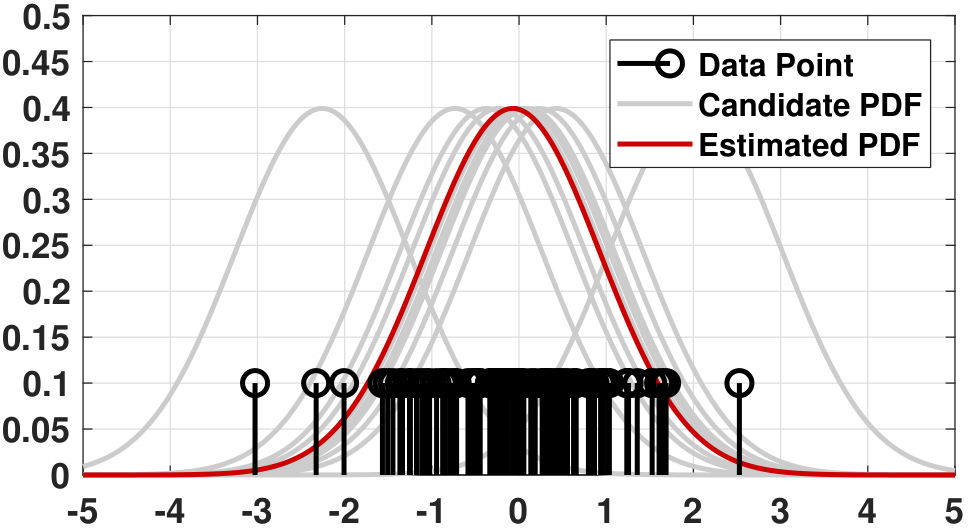
When \(N = 10\) and \(N = 100\). We can continue the above calculation for \(N =10\) and \(N =100\). In this case the MLE is

where the optimization is solved by taking the derivative: $$\frac{d}{d\theta} \sum_{n=1}^N (x_n-\theta)^2 = -2\sum_{n=1}^N (x_n-\theta)$$ Equating this with zero yields the solution \(\theta = \frac{1}{N}\sum_{n=1}^N x_n\).

The result suggests that for an arbitrary number of training samples the ML estimate is the sample average. These cases are illustrated in Figure 8.6. As you can see, the red curves (the estimated PDF) are always trying to fit as many data points as possible.

The above experiment tells us something about the ML estimation:

8.1.3Application 1: Social network analysis

ML estimation has extremely broad applicability. In this subsection and the next we discuss two real examples. We start with an example in social network analysis.

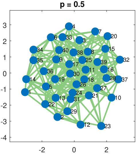
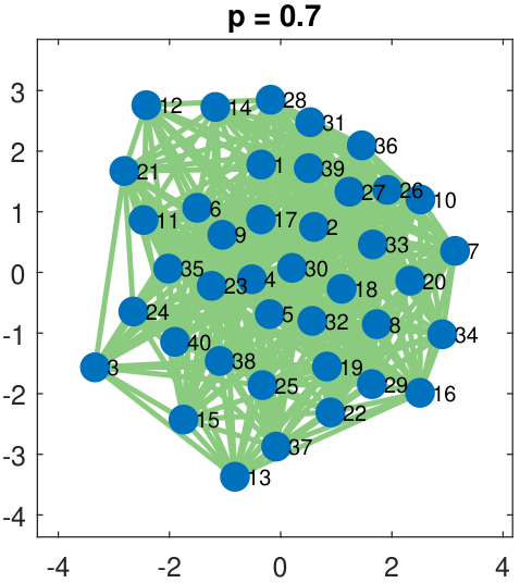
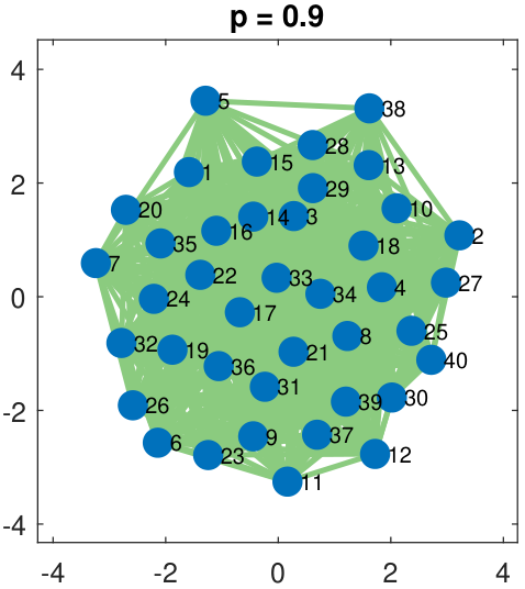
In Chapter 3, when we discussed the Bernoulli random variables, we introduced the Erdos-R\'enyi graph — one of the simplest models for social networks. The Erdos-R\'enyi graph is a single-membership network that assumes that all users belong to the same cluster. Thus the connectivity between users is specified by a single parameter, which is also the probability of the Bernoulli random variable.

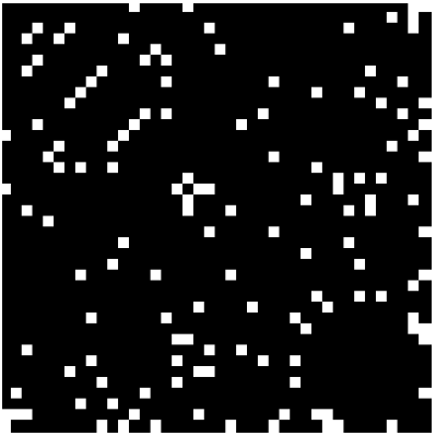
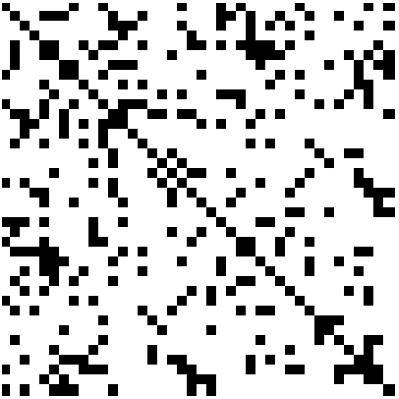
In our discussions in Chapter 3 we defined an adjacency matrix to represent a graph. The adjacency matrix is a binary matrix, with the \((i,j)\)th entry indicating an edge connecting nodes \(i\) and \(j\). Since the presence and absence of an edge is binary and random, we may model each element of the adjacency matrix as a Bernoulli random variable

In other words, the edge \(X_{ij}\) linking user \(i\) and user \(j\) in the network is either \(X_{ij} = 1\) with probability \(p\), or \(X_{ij} = 0\) with probability \(1-p\). In terms of notation, we define the matrix \(\mX \in \R^{N \times N}\) as the adjacency matrix, with the \((i,j)\)th element being \(X_{ij}\).

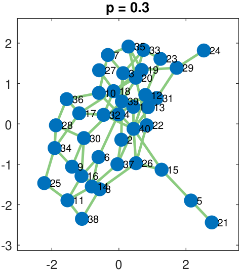
A few examples of a single-membership Erdos-R\'enyi graph are shown in Figure 8.7. As the figure shows, the network connectivity increases as the Bernoulli parameter \(p\) increases. This happens because \(p\) defines the “density” of the edges. If \(p\) is large, we have a greater chance of getting \(X_{ij} = 1\), and so there is a higher probability that an edge is present between node \(i\) and node \(j\). If \(p\) is small, the probability is lower.

Suppose that we are given one snapshot of the network, i.e., one realization \(\vx \in \R^{N \times N}\) of the adjacency matrix \(\mX \in \R^{N \times N}\). The problem of recovering the latent parameter \(p\) can be formulated as an ML estimation.

Now that we have the log-likelihood function, we can proceed to estimate the parameter \(p\). The solution to this is the ML estimate.

On computers, visualizing the graphs and computing the ML estimates are reasonably straightforward. In MATLAB, you can call the command graph to build a graph from the adjacency matrix A. This will allow you to plot the graph. The computation, however, is done directly by the adjacency matrix. In the code below, you can see that we call rand to generate the Bernoulli random variables. The command triu extracts the upper triangular matrix from the matrix A. This ensures that we do not pick the diagonals. The symmetrization of A+A' ensures that the graph is undirected, meaning that \(i\) to \(j\) is the same as \(j\) to \(i\).

% MATLAB code to visualize a graph
    n = 40;             % Number of nodes
    p = 0.3             % probability
    A = rand(n,n)<p;
    A = triu(A,1);
    A = A+A';           % Adj matrix
    G = graph(A);       % Graph
    plot(G);            % Drawing
    p_ML = mean(A(:));  % ML estimate

In Python, the computation is done similarly with the help of the networkx library. The number of edges m is defined as \(m = p \frac{n^2}{2}\). This is because for a graph with \(n\) nodes, there are at most \(\frac{n^2}{2}\) unique pairs of undirected edges. Multiplying this number by the probability \(p\) will give us the number of edges \(m\).

# Python code to visualize a graph
    import networkx as nx
    import numpy as np
    n = 40                       # Number of nodes
    p = 0.3                      # probability
    m = np.round(((n ** 2)/2)*p) # Number of edges
    G = nx.gnm_random_graph(n,m) # Graph
    A = nx.adjacency_matrix(G)   # Adj matrix
    nx.draw(G)                   # Drawing
    p_ML = np.mean(A)            # ML estimate

As you can see in both the MATLAB and the Python code, the ML estimate \(\widehat{p}_{\text{ML}}\) is determined by taking the sample average. Thus the ML estimate, according to our calculation, is \(\widehat{p}_{\text{ML}} = \frac{1}{N^2}\sum_{i=1}^N \sum_{j=1}^N x_{ij}\).

8.1.4Application 2: Reconstructing images

Being able to see in the dark is the holy grail of imaging. Many advanced sensing technologies have been developed over the past decade. In this example, we consider a single-photon image sensor. This is a counting device that counts the number of photons arriving at the sensor. Physicists have shown that a Poisson process can model the arrival of the photons. For simplicity we assume a homogeneous pattern of \(N\) pixels. The underlying intensity of the homogeneous pattern is a constant \(\lambda\).

Suppose that we have a sensor with \(N\) pixels \(X_1,\ldots,X_N\). According to the Poisson statistics, the probability of observing a pixel value is determined by the Poisson probability:

or more explicitly,

where \(x_{n}\) is the \(n\)th observed pixel value, and is an integer.

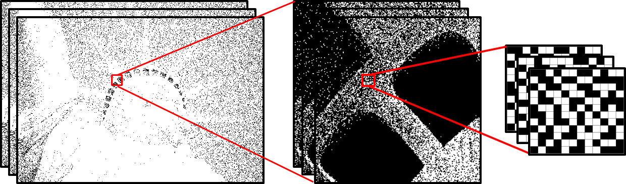
A single-photon image sensor is slightly more complicated in the sense that it does not report \(X_n\) but instead reports a truncated version of \(X_{n}\). Depending on the number of incoming photons, the sensor reports

We call this type of sensor a one-bit single-photon image sensor (see Figure 8.8). Our question is: If we are given the measurements \(Y_1,\ldots,Y_N\), can we estimate the underlying parameter \(\lambda\)?

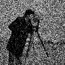
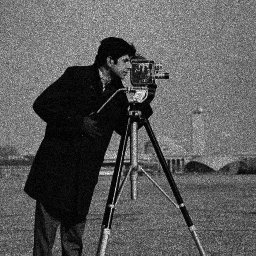
For real images, you can extrapolate the idea from \(y_n\) to \(y_{i,j,t}\), which denotes the \((i,j)\)th pixel located at time \(t\). Defining \(\vy_t \in \R^{N \times N}\) as the \(t\)th frame of the observed data, we can use \(T\) frames to recover one image \(\widehat{\vlambda}_{\text{ML}} \in \R^{N \times N}\). It follows from the above derivation that the ML estimate is

Figure 8.9 shows a pair of input-output images of a \(256\times 256\) image.

On a computer the ML estimation can be done in a few lines of MATLAB code. The code in Python requires more work, as it needs to read images using the openCV library.

% MATLAB code to recover an image from binary measurements
    lambda = im2double(imread('cameraman.tif'));
    T = 100;                                    % 100 frames
    x = poissrnd( repmat(lambda, [1,1,T]) );    % generate Poisson r.v.
    y = (x>=1);                                 % binary truncation
    lambdahat = -log(1-mean(y,3));              % ML estimation
    figure(1); imshow(x(:,:,1));
    figure(2); imshow(lambdahat);

# Python code to recover an image from binary measurements
    import cv2
    import numpy as np
    import scipy.stats as stats
    import matplotlib.pyplot as plt
    lambd = cv2.imread('./cameraman.tif')               # read image
    lambd = cv2.cvtColor(lambd, cv2.COLOR_BGR2GRAY)/255 # gray scale
    T = 100
    lambdT = np.repeat(lambd[:, :, np.newaxis], T, axis=2)  # repeat image
    x = stats.poisson.rvs(lambdT)                       # Poisson statistics
    y = (x>=1).astype(float)                            # binary truncation
    lambdhat = -np.log(1-np.mean(y,axis=2))             # ML estimation
    plt.imshow(lambdhat,cmap='gray')

8.1.5More examples of ML estimation

By now you should be familiar with the procedure for solving the ML estimation problem. We summarize the two steps as follows.

The idea of ML estimation can also be extended to vector observations.

8.1.6Regression versus ML estimation

ML estimation is closely related to regression. To understand the connection, we consider a linear model that we studied in Chapter 7. This model describes the relationship between the inputs \(\vx_1,\ldots,\vx_N\) and the observed outputs \(y_1,\ldots,y_N\), via the equation

In this expression, \(\phi_p(\cdot)\) is a transformation that extracts the “features” of the input vector \(\vx\) to produce a scalar. The coefficient \(\theta_p\) defines the relative weight of the feature \(\phi_p(\vx_n)\) in constructing the observed variable \(y_n\). The error \(e_n\) defines the modeling error between the observation \(y_n\) and the prediction \(\sum_{p=0}^{d-1} \theta_p\phi_p(\vx_n)\). We call this equation a linear model.

Expressed in matrix form, the linear model is

or more compactly as \(\vy = \mX\vtheta + \ve\). Rearranging the terms, it is easy to show that

Now we make an assumption: that each noise \(e_n\) is an i.i.d. copy of a Gaussian random variable with zero mean and variance \(\sigma^2\). In other words, the error vector \(\ve\) is distributed according to \(\ve \sim \text{Gaussian}(\vzero,\sigma^2\mI)\). This assumption is not always true because there are many situations in which the error is not Gaussian. However, this assumption is necessary for us to make the connection between ML estimation and regression.

With this assumption, we ask, given the observations \(y_1,\ldots,y_N\), what would be the ML estimate of the unknown parameter \(\vtheta\)? We answer this question in two steps.

The next step is to solve the ML estimation by maximizing the log-likelihood.

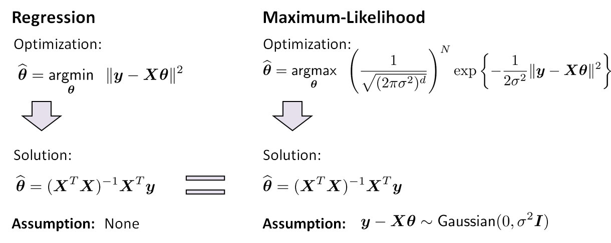
Since the ML estimate in Eq. (8.20) is the same as the regression solution (see Chapter 7), we conclude that the regression problem of a linear model is equivalent to solving an ML estimation problem.

The main difference between a linear regression problem and an ML estimation problem is the underlying statistical model, as illustrated in Figure 8.10. In linear regression, you do not care about the statistics of the noise term \(e_n\). We choose \((\cdot)^2\) as the error because it is differentiable and convenient. In ML estimation, we choose \((\cdot)^2\) as the error because the noise is Gaussian. If the noise is not Gaussian, e.g., the noise follows a Laplace distribution, we need to choose \(|\cdot|\) as the error. Therefore, you can always get a result by solving the linear regression. However, this result will only become meaningful if you provide additional information about the problem. For example, if you know that the noise is Gaussian, then the regression solution is also the ML solution. This is a statistical guarantee.

In practice, of course, we do not know whether the noise is Gaussian or not. At this point we have two courses of action: (i) Use your prior knowledge/domain expertise to determine whether a Gaussian assumption makes sense, or (ii) select an alternative model and see if the alternative model fits the data better. In practice, we should also question whether maximizing the likelihood is what we want. We may have some knowledge and therefore prefer the parameter \(\vtheta\), e.g., we want a sparse solution so that \(\vtheta\) only contains a few non-zeros. In that case, maximizing the likelihood without any constraint may not be the solution we want.