Linear Algebra
The two most important subjects for data science are probability, which is the subject of the book you are reading, and linear algebra, which concerns matrices and vectors. We cannot cover linear algebra in detail because this would require another book. However, we need to highlight some ideas that are important for doing data analysis.
1.4.1Why do we need linear algebra in data science?
Consider a dataset of the crime rate of several cities as shown below, downloaded from https://web.stanford.edu/ hastie/StatLearnSparsity/data.html.
The table shows that the crime rate depends on several factors such as funding for the police department, the percentage of high school graduates, etc.
| city | crime rate | funding | hs | no-hs | college | college4 |
| 1 | 478 | 40 | 74 | 11 | 31 | 20 |
| 2 | 494 | 32 | 72 | 11 | 43 | 18 |
| 3 | 643 | 57 | 71 | 18 | 16 | 16 |
| 4 | 341 | 31 | 71 | 11 | 25 | 19 |
| 50 | 940 | 66 | 67 | 26 | 18 | 16 |
What questions can we ask about this table? We can ask: What is the most influential cause of the crime rate? What are the leading contributions to the crime rate? To answer these questions, we need to describe these numbers. One way to do it is to put the numbers in matrices and vectors. For example,
With this vector expression of the data, the analysis questions can roughly be translated to finding \(\beta\)'s in the following equation:
This equation offers a lot of useful insights. First, it is a linear model of \(\vy_{\text{crime}}\). We call it a linear model because the observable \(\vy_{\text{crime}}\) is written as a linear combination of the variables \(\vx_{\text{fund}}, \vx_{\text{hs}}\), etc. The linear model assumes that the variables are scaled and added to generate the observed phenomena. This assumption is not always realistic, but it is often a fair assumption that greatly simplifies the problem. For example, if we can show that all \(\beta\)'s are zero except \(\beta_{\text{fund}}\), then we can conclude that the crime rate is solely dependent on the police funding. If two variables are correlated, e.g., high school graduate and college graduate, we would expect the \(\beta\)'s to change simultaneously.
The linear model can further be simplified to a matrix-vector equation:
Here, the lines “\(|\)” emphasize that the vectors are column vectors. If we denote the matrix in the middle as \(\mA\) and the vector as \(\vbeta\), then the equation is equivalent to \(\vy = \mA \vbeta\). So we can find \(\vbeta\) by appropriately inverting the matrix \(\mA\). If two columns of \(\mA\) are dependent, we will not be able to resolve the corresponding \(\beta\)'s uniquely.
As you can see from the above data analysis problem, matrices and vectors offer a way to describe the data. We will discuss the calculations in Chapter 7. However, to understand how to interpret the results from the matrix-vector equations, we need to review some basic ideas about matrices and vectors.
1.4.2Everything you need to know about linear algebra
Throughout this book, you will see different sets of notations. For linear algebra, we also have a set of notations. We denote \(\vx \in \R^d\) as a \(d\)-dimensional vector taking real numbers as its entries. An \(M\)-by-\(N\) matrix is denoted as \(\mX \in \R^{M \times N}\). The transpose of a matrix is denoted as \(\mX^T\). A matrix \(\mX\) can be viewed according to its columns and its rows:
Here, \(\vx_j\) denotes the \(j\)th column of \(\mX\), and \(\vx^i\) denotes the \(i\)th row of \(\mX\). The \((i,j)\)th element of \(\mX\) is denoted as \(x_{ij}\) or \([\mX]_{ij}\). The identity matrix is denoted as \(\mI\). The \(i\)th column of \(\mI\) is denoted as \(\ve_i = [0,\ldots,1,\ldots,0]^T\), and is called the \(i\)th standard basis vector. An all-zero vector is denoted as \(\vzero = [0,\ldots,0]^T\).
What is the most important thing to know about linear algebra? From a data analysis point of view, Figure 1.11 gives us the answer. The picture is straightforward, but it captures all the essence. In almost all the data analysis problems, ultimately, there are three things we care about: (i) The observable vector \(\vy\), (ii) the variable vectors \(\vx_n\), and (iii) the coefficients \(\beta_n\). The set of variable vectors \(\{\vx_n\}_{n=1}^N\) spans a vector space in which all vectors live. Some of these variable vectors are correlated, and some are not. However, for the sake of this discussion, let us assume they are independent of each other. Then for any observable vector \(\vy\), we can always project \(\vy\) in the directions determined by \(\{\vx_n\}_{n=1}^N\). The projection of \(\vy\) onto \(\vx_n\) is the coefficient \(\beta_n\). A larger value of \(\beta_n\) means that the variable \(\vx_n\) has more contributions.
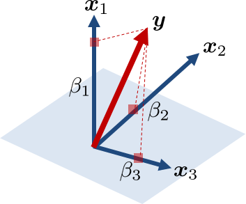
Why is this picture so important? Because most of the data analysis problems can be expressed, or approximately expressed, by the picture:
If you recall the crime rate example, this equation is precisely the linear model we used to describe the crime rate. This equation can also describe many other problems.
Polynomial fitting. Consider a dataset of pairs of numbers \((t_m,y_m)\) for \(m = 1,\ldots,M\), as shown in Figure 1.12. After a visual inspection of the dataset, we propose to use a line to fit the data. A line is specified by the equation
where \(a \in \R\) is the slope and \(b \in \R\) is the \(y\)-intercept. The goal of this problem is to find one line (which is fully characterized by \((a,b)\)) such that it has the best fit to all the data pairs \((t_m,y_m)\) for \(m = 1,\ldots,M\). This problem can be described in matrices and vectors by noting that
or more compactly,
Here, \(\vx_1 = [t_1,\ldots,t_M]^T\) contains all the variable values, and \(\vx_2 = [1,\ldots,1]^T\) contains a constant offset.
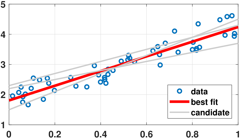
Image compression. The JPEG compression for images is based on the concept of discrete cosine transform (DCT). The DCT consists of a set of basis vectors, or \(\{\vx_n\}_{n=1}^N\) using our notation. In the most standard setting, each basis vector \(\vx_n\) consists of \(8 \times 8\) pixels, and there are \(N = 64\) of these \(\vx_n\)'s. Given an image, we can partition the image into \(M\) small blocks of \(8 \times 8\) pixels. Let us call one of these blocks \(\vy\). Then, DCT represents the observation \(\vy\) as a linear combination of the DCT basis vectors:
The coefficients \(\{\beta_n\}_{n=1}^N\) are called the DCT coefficients. They provide a representation of \(\vy\), because once we know \(\{\beta_n\}_{n=1}^N\), we can completely describe \(\vy\) because the basis vectors \(\{\vx_n\}_{n=1}^N\) are known and fixed. The situation is depicted in Figure 1.13.
How can we compress images using DCT? In the 1970s, scientists found that most images have strong leading DCT coefficients but weak tail DCT coefficients. In other words, among the \(N=64\) \(\beta_n\)'s, only the first few are important. If we truncate the number of DCT coefficients, we can effectively compress the number of bits required to represent the image.

We hope by now you are convinced of the importance of matrices and vectors in the context of data science. They are not “yet another” subject but an essential tool you must know how to use. So, what are the technical materials you must master? Here we go.
1.4.3Inner products and norms
We assume that you know the basic operations such as matrix-vector multiplication, taking the transpose, etc. If you have forgotten these, please consult any undergraduate linear algebra textbook such as Gilbert Strang's Linear Algebra and its Applications. We will highlight a few of the most important operations for our purposes.
Let \(\vx = [x_1, \ldots, x_N]^T\), and \(\vy = [y_1, \ldots, y_N]^T\). The inner product \(\vx^T\vy\) is
Let \(\vx = [1, \; 0, \; -1]^T\), and \(\vy = [3, \; 2, \; 0]^T\). Find \(\vx^T\vy\).
The inner product is \(\vx^T\vy = (1)(3) + (0)(2) + (-1)(0) = 3\).
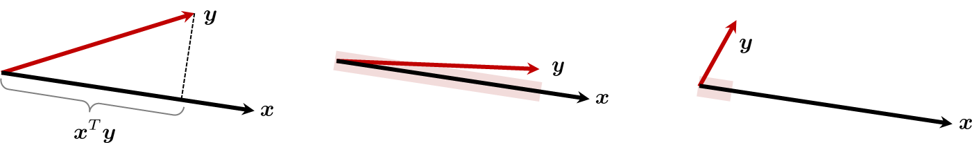
Inner products are important because they tell us how two vectors are correlated. Figure 1.14 depicts the geometric meaning of an inner product. If two vectors are correlated (i.e., nearly parallel), then the inner product will give us a large value. Conversely, if the two vectors are close to perpendicular, then the inner product will be small. Therefore, the inner product provides a measure of the closeness/similarity between two vectors.
Creating vectors and computing the inner products are straightforward in MATLAB. We simply need to define the column vectors x and y by using the command [] with ; to denote the next row. The inner product is done using the transpose operation x' and vector multiplication *.
% MATLAB code to perform an inner product
    x = [1 0 -1];
    y = [3 2 0];
    z = x'*y;
In Python, constructing a vector is done using the command np.array. Inside this command, one needs to enter the array. For a column vector, we write [[1],[2],[3]], with an outer [], and three inner [] for each entry. If the vector is a row vector, then one can omit the inner []'s by just calling np.array([1, 2, 3]). Given two column vectors x and y, the inner product is computed via np.dot(x.T,y), where np.dot is the command for inner product, and x.T returns the transpose of x. One can also call np.transpose(x), which is the same as x.T.
# Python code to perform an inner product
    import numpy as np
    x = np.array([[1],[0],[-1]])
    y = np.array([[3],[2],[0]])
    z = np.dot(np.transpose(x),y)
    print(z)
In data analytics, the inner product of two vectors can be useful. Consider the vectors in Table 1.2. Just from looking at the numbers, you probably will not see anything wrong. However, let's compute the inner products. It turns out that \(\vx_1^T\vx_2 = -0.0031\), whereas \(\vx_1^T\vx_3 = 2.0020\). There is almost no correlation between \(\vx_1\) and \(\vx_2\), but there is a substantial correlation between \(\vx_1\) and \(\vx_3\). What happened? The vectors \(\vx_1\) and \(\vx_2\) are random vectors constructed independently and uncorrelated with each other. The last vector \(\vx_3\) was constructed by \(\vx_3 = 2\vx_1 - \pi/1000\). Since \(\vx_3\) is completely constructed from \(\vx_1\), they have to be correlated.
| \(\vx_1\) | \(\vx_2\) | \(\vx_3\) |
| \(0.0006\) | \(-0.0011\) | \(-0.0020\) |
| \(-0.0014\) | \(-0.0024\) | \(-0.0059\) |
| \(-0.0034\) | \(0.0073\) | \(-0.0099\) |
| \(0.0001\) | \(-0.0066\) | \(-0.0030\) |
| \(0.0074\) | \(0.0046\) | \(0.0116\) |
| \(0.0007\) | \(-0.0061\) | \(-0.0017\) |
One caveat for this example is that the naive inner product \(\vx_i^T\vx_j\) is scale-dependent. For example, the vectors \(\vx_3 = \vx_1\) and \(\vx_3 = 1000\vx_1\) have the same amount of correlation, but the simple inner product will give a larger value for the latter case. To solve this problem, we first define the norm of the vectors:
Let \(\vx = [x_1, \ldots, x_N]^T\) be a vector. The \(\ell_p\)-norm of \(\vx\) is
for any \(p \ge 1\).
The norm essentially tells us the length of the vector. This is most obvious if we consider the \(\ell_2\)-norm:
By squaring both sides, one can show that \(\|\vx\|_2^2 = \vx^T\vx\). This is called the squared \(\ell_2\)-norm, and is the sum of the squares.
On MATLAB, computing the norm is done using the command norm. Here, we can indicate the types of norms, e.g., norm(x,1) returns the \(\ell_1\)-norm whereas norm(x,2) returns the \(\ell_2\)-norm (which is also the default).
% MATLAB code to compute the norm
    x = [1 0 -1];
    x_norm = norm(x);
On Python, the norm command is listed in the np.linalg. To call the \(\ell_1\)-norm, we use np.linalg.norm(x,1), and by default the \(\ell_2\)-norm is np.linalg.norm(x).
# Python code to compute the norm
    import numpy as np
    x = np.array([[1],[0],[-1]])
    x_norm = np.linalg.norm(x)
Using the norm, one can define an angle called the cosine angle between two vectors.
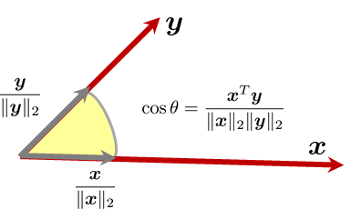
The cosine angle between two vectors \(\vx\) and \(\vy\) is
The difference between the cosine angle and the basic inner product is the normalization in the denominator, which is the product \(\|\vx\|_2\|\vy\|_2\). This normalization factor scales the vector \(\vx\) to \(\vx/\|\vx\|_2\) and \(\vy\) to \(\vy/\|\vy\|_2\). The scaling makes the length of the new vector equal to unity, but it does not change the vector's orientation. Therefore, the cosine angle is not affected by a very long vector or a very short vector. Only the angle matters. See Figure 1.15.
Going back to the previous example, after normalization, we can show that the cosine angle between \(\vx_1\) and \(\vx_2\) is \(\cos\theta_{1,2} = -0.0031\), whereas the cosine angle between \(\vx_1\) and \(\vx_3\) is \(\cos\theta_{1,3} = 0.8958\). There is still a strong correlation between \(\vx_1\) and \(\vx_3\), but now using the cosine angle the value is between \(-1\) and \(+1\).
Remark 1: There are other norms one can use. The \(\ell_1\)-norm is useful for sparse models where we want to have the fewest possible non-zeros. The \(\ell_1\)-norm of \(\vx\) is
which is the sum of absolute values. The \(\ell_{\infty}\)-norm picks the maximum of \(\{|x_1|,\ldots,|x_N|\}\):
because as \(p \rightarrow \infty\), only the largest element will be amplified.
Remark 2: The standard \(\ell_2\)-norm is a circle: Just consider \(\vx = [x_1,x_2]^T\). The norm is \(\|\vx\|_2 = \sqrt{x_1^2+x_2^2}\). We can convert the circle to ellipses by considering a weighted norm.
Let \(\vx = [x_1, \ldots, x_N]^T\) and let \(\mW = \mbox{diag}(w_1,\ldots,w_N)\) be a non-negative diagonal matrix. The weighted \(\ell_2\)-norm square of \(\vx\) is
The geometry of the weighted \(\ell_2\)-norm is determined by the matrix \(\mW\). For example, if \(\mW = \mI\) (the identity operator), then \(\|\vx\|_{\mW}^2 = \|\vx\|_2^2\), which defines a circle. If \(\mW\) is any “non-negative” matrix (The technical term for these matrices is positive semi-definite matrices.), then \(\|\vx\|_{\mW}^2\) defines an ellipse.
In MATLAB, the weighted inner product is just a sequence of two matrix-vector multiplications. This can be done using the command x'*W*x as shown below.
% MATLAB code to compute the weighted norm
    W = [1 2 3; 4 5 6; 7 8 9];
    x = [2; -1; 1];
    z = x'*W*x
In Python, constructing the matrix \(\mW\) and the column vector \(\vx\) is done using np.array. The matrix-vector multiplication is done using two np.dot commands: one for np.dot(W,x) and the other one for np.dot(x.T, np.dot(W,x)).
# Python code to compute the weighted norm
    import numpy as np
    W = np.array([[1, 2, 3], [4, 5, 6], [7, 8, 9]])
    x = np.array([[2],[-1],[1]])
    z = np.dot(x.T, np.dot(W,x))
print(z)1.4.4Matrix calculus
The last linear algebra topic we need to review is matrix calculus. As its name indicates, matrix calculus is about the differentiation of matrices and vectors. Why do we need differentiation for matrices and vectors? Because we want to find the minimum or maximum of a scalar function with a vector input.
Let us go back to the crime rate problem we discussed earlier. Given the data, we want to find the model coefficients \(\beta_1,\ldots,\beta_N\) such that the variables can best explain the observation. In other words, we want to minimize the deviation between \(\vy\) and the prediction offered by our model:
This equation is self-explanatory. The norm \(\|\clubsuit-\heartsuit\|^2\) measures the deviation. If \(\vy\) can be perfectly explained by \(\{\vx_n\}_{n=1}^N\), then the norm can eventually go to zero by finding a good set of \(\{\beta_1,\ldots,\beta_N\}\). The symbol \(\minimize{\beta_1,\ldots,\beta_N}\) means to minimize the function by finding \(\{\beta_1,\ldots,\beta_N\}\). Note that the norm is taking a vector as the input and generating a scalar as the output. It can be expressed as
to emphasize this relationship. Here we define \(\vbeta = [\beta_1,\ldots,\beta_N]^T\) as the collection of all coefficients.
Given this setup, how would you determine \(\vbeta\) such that the deviation is minimized? Our calculus teachers told us that we could take the function's derivative and set it to zero for scalar problems. It is the same story for vectors. What we do is to take the derivative of the error and set it equal to zero:
Now the question arises, how do we take the derivatives of \(\varepsilon(\vbeta)\) when it takes a vector as input? If we can answer this question, we will find the best \(\vbeta\). The answer is straightforward. Since the function has one output and many inputs, take the derivative for each element independently. This is called the scalar differentiation of vectors.
Let \(f: \R^N \rightarrow \R\) be a differentiable scalar function, and let \(y = f(\vx)\) for some input \(\vx \in \R^N\). Then,
As you can see from this definition, there is nothing conceptually challenging here. The only difficulty is that things can get tedious because there will be many terms. However, the good news is that mathematicians have already compiled a list of identities for common matrix differentiation. So instead of deriving every equation from scratch, we can enjoy the fruit of their hard work by referring to those formulae. The best place to find these equations is the Matrix Cookbook by Petersen and Pedersen. (https://www.math.uwaterloo.ca/ hwolkowi/matrixcookbook.pdf) Here, we will mention two of the most useful results.
Let \(y = \vx^T\mA\vx\) for any matrix \(\mA \in \R^{N \times N}\). Find \(\frac{d y}{d\vx}\).
Now, if \(\mA\) is symmetric, i.e., \(\mA = \mA^T\), then
Let \(\varepsilon = \|\mA\vx - \vy\|_2^2\), where \(\mA \in \R^{N \times N}\) is symmetric. Find \(\frac{d \varepsilon}{d\vx}\).
First, we note that
Taking the derivative with respect to \(\vx\) yields
Going back to the crime rate problem, we can now show that
Therefore, the solution is
As you can see, if we do not have access to the matrix calculus, we will not be able to solve the minimization problem. (There are alternative paths that do not require matrix calculus, but they require an understanding of linear subspaces and properties of the projection operators. So in some sense, matrix calculus is the easiest way to solve the problem.) When we discuss the linear regression methods in Chapter 7, we will cover the interpretation of the inverses and related topics.
In MATLAB and Python, matrix inversion is done using the command inv in MATLAB and np.linalg.inv in Python. Below is an example in Python.
# Python code to compute a matrix inverse
    import numpy as np
    X      = np.array([[1, 3], [-2, 7], [0, 1]])
    XtX    = np.dot(X.T, X)
    XtXinv = np.linalg.inv(XtX)
    print(XtXinv)
Sometimes, instead of computing the matrix inverse we are more interested in solving a linear equation \(\mX\vbeta = \vy\) (the solution of which is \(\widehat{\vbeta} = (\mX^T\mX)^{-1}\mX^T\vy\)). In both MATLAB and Python, there are built-in commands to do this. In MATLAB, the command is \ (backslash).
% MATLAB code to solve X beta = y
    X      = [1 3; -2 7; 0 1];
    y      = [2; 1; 0];
    beta   = X\y;
In Python, the built-in command is np.linalg.lstsq.
# Python code to solve X beta = y
    import numpy as np
    X      = np.array([[1, 3], [-2, 7], [0, 1]])
    y      = np.array([[2],[1],[0]])
    beta   = np.linalg.lstsq(X, y, rcond=None)[0]
    print(beta)
Closing remark: In this section, we have given a brief introduction to a few of the most relevant concepts in linear algebra. We will introduce further concepts in linear algebra in later chapters, such as eigenvalues, principal component analysis, linear transformations, and regularization, as they become useful for our discussion.