eBook › Chapter 3 · Discrete Random Variables

Section 3.1

Random Variables

3.1.1A motivating example

Consider an experiment with 4 outcomes $\Omega = \{\clubsuit,\diamondsuit,\heartsuit,\spadesuit\}$. We want to construct the probability space $(\Omega, \calF, \Pb)$. The sample space $\Omega$ is already defined. The event space $\calF$ is the set of all possible subsets in $\Omega$, which, in our case, is a set of $2^4$ subsets. For the probability law $\Pb$, let us assume that the probability of obtaining each outcome is

\begin{aligned} \Pb[\{\clubsuit\}] = \frac{1}{6}, \quad \Pb[\{\diamondsuit\}] = \frac{2}{6}, \quad \Pb[\{\heartsuit\}] = \frac{2}{6}, \quad \Pb[\{\spadesuit\}] = \frac{1}{6}. \end{aligned}

Therefore, we have constructed a probability space $(\Omega, \calF, \Pb)$ where everything is perfectly defined. So, in principle, they can live together happily forever.

A lazy data scientist comes, and there is a (small) problem. The data scientist does not want to write the symbols $\clubsuit,\diamondsuit,\heartsuit,\spadesuit$. There is nothing wrong with his motivation because all of us want efficiency. How can we help him? Well, the easiest solution is to encode each symbol with a number, for example, $\clubsuit \leftarrow 1$, $\diamondsuit \leftarrow 2$, $\heartsuit \leftarrow 3$, $\spadesuit \leftarrow 4$, where the arrow means that we assign a number to the symbol. But we can express this more formally by defining a function $X: \Omega \rightarrow \R$ with

\begin{aligned} X(\clubsuit) = 1, \;\; X(\diamondsuit) = 2, \;\; X(\heartsuit) = 3, \;\; X(\spadesuit) = 4. \end{aligned}

There is nothing new here: we have merely converted the symbols to numbers, with the help of a function $X$. However, with $X$ defined, the probabilities can be written as

\begin{aligned} \Pb[X = 1] = \frac{1}{6}, \quad \Pb[X = 2] = \frac{2}{6}, \quad \Pb[X = 3] = \frac{2}{6}, \quad \Pb[X = 4] = \frac{1}{6}. \end{aligned}

This is much more convenient, and so the data scientist is happy.

3.1.2Definition of a random variable

The story above is exactly the motivation for random variables. Let us define a random variable formally.

Definition 3.1

A random variable $X$ is a function $X: \Omega \rightarrow \R$ that maps an outcome $\xi \in \Omega$ to a number $X(\xi)$ on the real line.

This definition may be puzzling at first glance. Why should we overcomplicate things by defining a function and calling it a variable?

If you recall the story above, we can map the notations of the story to the notations of the definition as follows.

Symbol	Meaning
$\Omega$	sample space = the set containing $\clubsuit,\diamondsuit,\heartsuit,\spadesuit$
$\xi$	an element in the sample space, which is one of $\clubsuit,\diamondsuit,\heartsuit,\spadesuit$
$X$	a function that maps $\clubsuit$ to the number 1, $\diamondsuit$ to the number 2, etc
$X(\xi)$	a number on the real line, e.g., $X(\clubsuit) = 1$

This explains our informal definition of random variables:

Key Concept 1: What are random variables?

Random variables are mappings from outcomes to numbers.

The random variable $X$ is a function. The input to the function is an outcome of the sample space, whereas the output is a number on the real line. This type of function is somewhat different from an ordinary function that often translates a number to another number. Nevertheless, $X$ is a function.

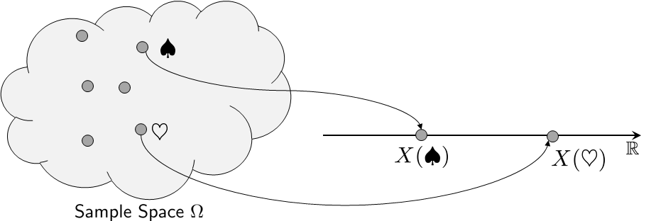
Why do we call this function $X$ a variable? $X$ is a variable because $X$ has multiple states. As we illustrate in Figure 3.1, the mapping $X$ translates every outcome $\xi$ to a number. There are multiple numbers, which are the states of $X$. Each state has a certain probability for $X$ to land on. Because $X$ is not deterministic, we call it a random variable.

Example 3.1

Suppose we flip a fair coin so that $\Omega = \{\text{head},\text{tail}\}$. We can define the random variable $X: \Omega \rightarrow \R$ as

\begin{aligned} X(\text{head}) = 1, \qquad\text{and}\qquad X(\text{tail}) = 0. \end{aligned}

Therefore, when we write $\Pb[X = 1]$ we actually mean $\Pb[\{\text{head}\}]$. Is there any difference between $\Pb[\{\text{head}\}]$ and $\Pb[X = 1]$? No, because they are describing two identical events. Note that the assignment of the value is totally up to you. You can say “head” is equal to the value 102. This is allowed and legitimate, but it isn't very convenient.

Example 3.2

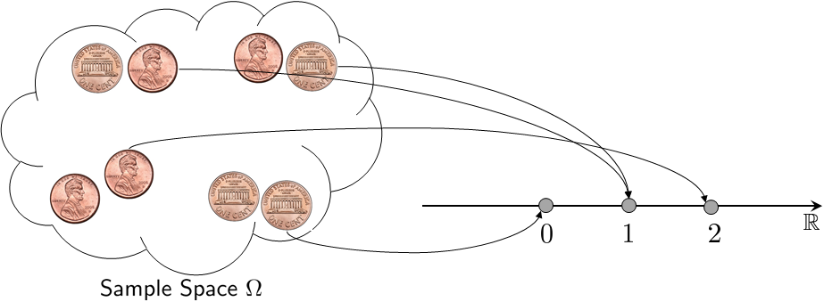
Flip a coin 2 times. The sample space $\Omega$ is

\begin{aligned} \Omega = \{(\text{head}, \text{head}),(\text{head}, \text{tail}),(\text{tail}, \text{head}),(\text{tail}, \text{tail})\}. \end{aligned}

Suppose that $X$ is a random variable that maps an outcome to a number representing the sum of “head,” i.e.,

X(\cdot) = \text{number of heads}.

Then, for the 4 $\xi$'s in the sample space there are only 3 distinct numbers. More precisely, if we let $\xi_1 = (\text{head}, \text{head})$, $\xi_2 = (\text{head}, \text{tail})$, $\xi_3 = (\text{tail}, \text{head})$, $\xi_4 = (\text{tail}, \text{tail})$, then, we have

\begin{aligned} X(\xi_1) = 2, \;\; X(\xi_2) = 1, \;\; X(\xi_3) = 1, \;\; X(\xi_4) = 0. \end{aligned}

A pictorial illustration of this random variable is shown in Figure 3.2. This example shows that the mapping defined by the random variable is not necessarily a one-to-one mapping because multiple outcomes can be mapped to the same number.

3.1.3Probability measure on random variables

By now, we hope that you understand Key Concept 1: A random variable is a mapping from a statement to a number. However, we are now facing another difficulty. We knew how to measure the size of an event using the probability law $\Pb$ because $\Pb(\cdot)$ takes an event $E \in \calF$ and sends it to a number between $[0,1]$. After the translation $X$, we cannot send the output $X(\xi)$ to $\Pb(\cdot)$ because $\Pb(\cdot)$ “eats” a set $E \in \calF$ and not a number $X(\xi) \in \R$. Therefore, when we write $\Pb[X = 1]$, how do we measure the size of the event $X = 1$?

This question appears difficult but is actually quite easy to answer. Since the probability law $\Pb(\cdot)$ is always applied to an event, we need to define an event for the random variable $X$. If we write the sets clearly, we note that “$X = a$” is equivalent to the set $$E = \bigg\{\xi \in \Omega \,\bigg|\, X(\xi) = a\bigg\}.$$ This is the set that contains all possible $\xi$'s such that $X(\xi) = a$. Therefore, when we say “find the probability of $X = a$,” we are effectively asking the size of the set $E = \{\xi \in \Omega \,|\, X(\xi) = a\}$.

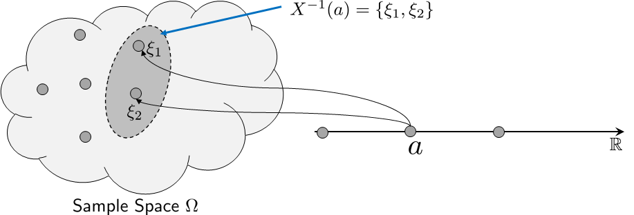
How then do we measure the size of $E$? Since $E$ is a subset in the sample space, $E$ is measurable by $\Pb$. All we need to do is to determine what $E$ is for a given $a$. This, in turn, requires us to find the pre-image $X^{-1}(a)$, which is defined as

X^{-1}(a) \bydef \bigg\{\xi \in \Omega \,\bigg|\, X(\xi) = a\bigg\}.

Wait a minute, is this set just equal to $E$? Yes, the event $E$ we are seeking is exactly the pre-image $X^{-1}(a)$. As such, the probability measure of $E$ is

\Pb[X = a] = \Pb[X^{-1}(a)].

Figure 3.3 illustrates a situation where two outcomes $\xi_1$ and $\xi_2$ are mapped to the same value $a$ on the real line. The corresponding event is the set $X^{-1}(a) = \{\xi_1,\xi_2\}$.

Example 3.3

Suppose we throw a die. The sample space is $$\Omega = \{\mydice{1}, \mydice{2},\mydice{3},\mydice{4},\mydice{5},\mydice{6}\}.$$ There is a natural mapping $X$ that maps $X(\mydice{1}) = 1$, $X(\mydice{2}) = 2$ and so on. Thus,

\begin{aligned} \Pb[X \le 3] &\overset{(a)}{=} \Pb[X = 1] + \Pb[X = 2] + \Pb[X = 3]\\ &\overset{(b)}{=} \Pb[X^{-1}(1)] + \Pb[X^{-1}(2)] + \Pb[X^{-1}(3)]\\ &\overset{(c)}{=} \Pb[\{\mydice{1}\}] + \Pb[\{\mydice{2}\}] + \Pb[\{\mydice{3}\}] = \frac{3}{6}. \end{aligned}

In this derivation, step (a) is based on Axiom III, where the three events are disjoint. Step (b) is the pre-image due to the random variable $X$. Step (c) is the list of actual events in the event space. Note that there is no hand-waving argument in this derivation. Every step is justified by the concepts and theorems we have learned so far.

Example 3.4

Throw a die twice. The sample space is then $$\Omega = \{(\mydice{1},\mydice{1}), (\mydice{1},\mydice{2}), \ldots, (\mydice{6},\mydice{6})\}.$$ These elements can be translated to 36 outcomes: $$\xi_1 = (\mydice{1},\mydice{1}), \xi_2 = (\mydice{1},\mydice{2}), \ldots, \xi_{36} = (\mydice{6},\mydice{6}).$$ Let $$X = \text{sum of two numbers}.$$ Then, if we want to find the probability of getting $X = 7$, we can trace back and ask: Among the 36 outcomes, which of those $\xi_i$'s will give us $X(\xi) = 7$? Or, what is the set $X^{-1}(7)$? To this end, we can write

\begin{aligned} \Pb[X = 7] &= \Pb[\{(\mydice{1},\mydice{6}), (\mydice{2},\mydice{5}), (\mydice{3},\mydice{4}), (\mydice{4},\mydice{3}), (\mydice{5},\mydice{2}), (\mydice{6},\mydice{1})\}]\\ &= \Pb[(\mydice{1},\mydice{6})] + \Pb[(\mydice{2},\mydice{5})] + \Pb[(\mydice{3},\mydice{4})] \\ &\qquad + \Pb[(\mydice{4},\mydice{3})] + \Pb[(\mydice{5},\mydice{2})] + \Pb[ (\mydice{6},\mydice{1})]\\ &= \frac{1}{36} + \frac{1}{36} + \frac{1}{36} + \frac{1}{36} + \frac{1}{36} + \frac{1}{36} = \frac{1}{6}. \end{aligned}

Again, in this example, you can see that all the steps are fully justified by the concepts we have learned so far.

Closing remark. In practice, when the problem is clearly defined, we can skip the inverse mapping $X^{-1}(a)$. However, this does not mean that the probability triplet $(\Omega,\calF,\Pb)$ is gone; it is still present. The triplet is now just the background of the problem.

The set of all possible values returned by $X$ is denoted as $X(\Omega)$. Since $X$ is not necessarily a bijection, the size of $X(\Omega)$ is not necessarily the same as the size of $\Omega$. The elements in $X(\Omega)$ are often denoted as $a$ or $x$. We call $a$ or $x$ one of the states of $X$. Be careful not to confuse $x$ with $X$. The variable $X$ is the random variable; it is a function. The variable $x$ is a state assigned by $X$. A random variable $X$ has multiple states. When we write $\Pb[X = x]$, we describe the probability of a random variable $X$ taking a particular state $x$. It is exactly the same as $\Pb[\{\xi \in \Omega \,|\, X(\xi) = x\}]$.

Symbol	Meaning
\(\Omega\)	sample space = the set containing \(\clubsuit,\diamondsuit,\heartsuit,\spadesuit\)
\(\xi\)	an element in the sample space, which is one of \(\clubsuit,\diamondsuit,\heartsuit,\spadesuit\)
\(X\)	a function that maps \(\clubsuit\) to the number 1, \(\diamondsuit\) to the number 2, etc
\(X(\xi)\)	a number on the real line, e.g., \(X(\clubsuit) = 1\)