eBook › Chapter 10 · Random Processes

Section 10.1

Basic Concepts

10.1.1Everything you need to know about a random process

Here is the single most important thing you need to remember about random processes:

What is a random process?

A random process is a function indexed by a random key.

That's it. Now you may be wondering what exactly a “function indexed by a random key” means. To help you see the picture, we consider two examples.

Example 10.1

We consider a set of straight lines. We define two random variables $a$ and $b$ that are uniformly distributed in a certain range. We then define a function:

f(t) = at + b, \qquad -2 \le t \le 2.

Clearly, $f(t)$ is a function of time $t$. But since $a$ and $b$ are random, $f(t)$ is also random. The randomness is caused by $a$ and $b$. To emphasize this dependency, we write $f(t)$ as

f(t, \xi) = a(\xi) t + b(\xi), \qquad -2 \le t \le 2,

where $\xi \in \Omega$ denotes the random index of the constants $(a,b)$ and $\Omega$ is the sample space of $\xi$. Therefore, by picking a different pair of constants $(a(\xi),b(\xi))$, we will have a different function $f(t,\xi)$, which in our case is a straight line of different slope and $y$-intercept.

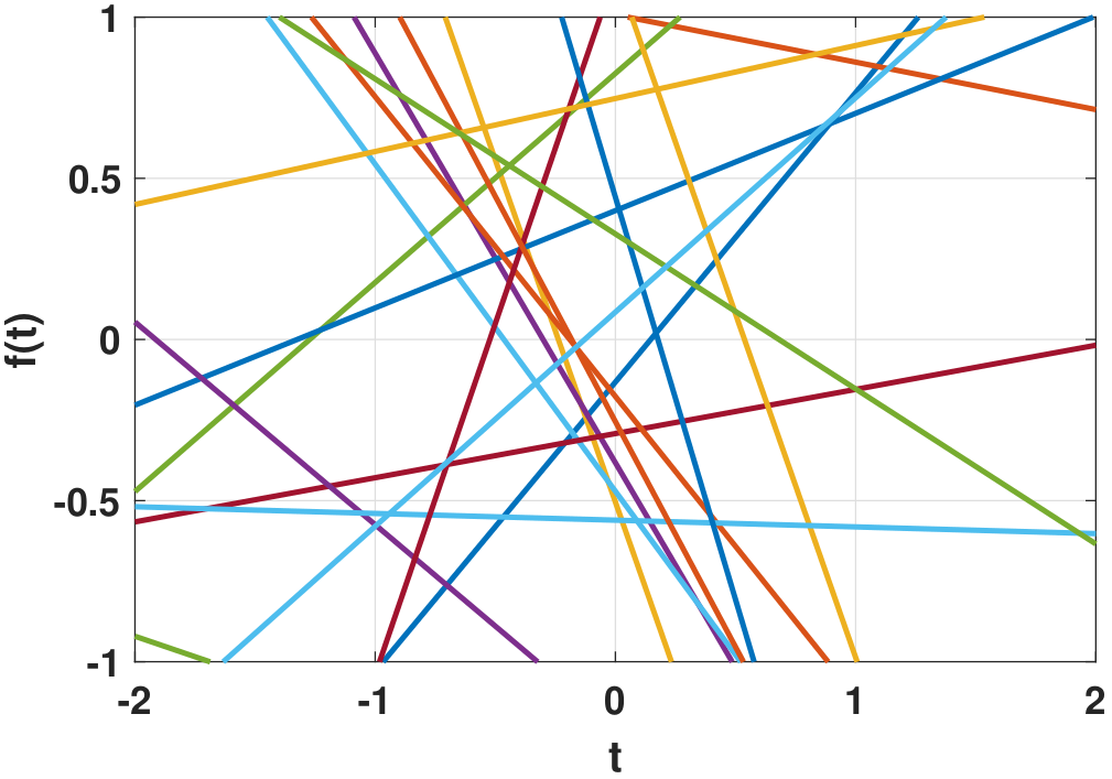
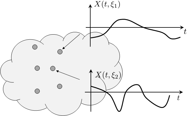
**Figure 10.1.** The set of straight lines $f(x) = ax+b$ where $a, b \in \R$.

As a special case of the example, suppose that the sample space contains only two pairs of constants: $(a,b) = (1.2, 0.6)$ and $(a,b) = (-0.75, 1.8)$. The probability of getting either pair is $\frac{1}{2}$. Then the function $f(t,\xi)$ will take two forms:

f(t,\xi) = \begin{cases} 1.2t + 0.6, &\qquad \text{with probability } \frac{1}{2},\\ -0.75t + 1.8, &\qquad \text{with probability } \frac{1}{2}. \end{cases}

Every time you pick a sample you pick one of the two functions, either $f(t,\xi_1)$ or $f(t,\xi_2)$. So we say that $f(t,\xi)$ is a random process because it is a function $f(t)$ indexed by a random key $\xi$.

Example 10.2

This example studies the function

f(t) = \cos(\omega_0 t + \Theta), \qquad -1 \le t \le 1,

where $\Theta$ is a random phase distributed uniformly over the range $[0,2\pi]$. Depending on the randomness of $\Theta$, the function $f(t)$ will take a different phase offset. To emphasize this dependency, we write

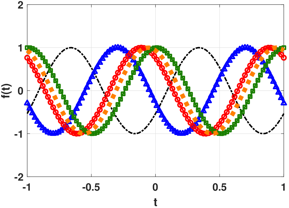
f(t,\xi) = \cos(\omega_0 t + \Theta(\xi)), \qquad -1 \le t \le 1.

**Figure 10.2.** The set of phase-shifted cosines $f(t) = \cos(\omega_0 t + \theta)$ where $\theta \in [0,2\pi]$.

Again, $\xi$ denotes the index of the random variable $\Theta$. Since $\Theta$ is drawn uniformly from the interval $[0,2\pi]$, the following functions are two possible realizations:

\begin{aligned} f(t,\xi_1) &= \cos\left(\omega_0 t + \frac{3\pi}{4}\right), \qquad -1 \le t \le 1,\\ f(t,\xi_2) &= \cos\left(\omega_0 t - \frac{7\pi}{3}\right), \qquad -1 \le t \le 1. \end{aligned}

Just as with the previous example, $f(t)$ is a function indexed by a random key $\xi$.

These two examples should give you a feeling for what to expect from a random process. A random process is quite similar to a random variable because they are both contained in a certain sample space. For (discrete) random variables, the sample space is a collection of outcomes $\{\xi_1,\xi_2,\ldots,\xi_N\}$. The random variable $X: \calF \rightarrow \R$ is a mapping that maps $\xi_n$ to $X(\xi_n)$, where $X(\xi_n)$ is a number. For random processes, the sample space is also $\{\xi_1,\xi_2,\ldots,\xi_N\}$. However, the mapping $X$ does not map $\xi_n$ to a number $X(\xi_n)$ but to a function $X(t,\xi_n)$. A function has the time index $t$, which is absent in the number. Therefore, for the same $\xi_n$, $X(t_1,\xi_n)$ can take one value and $X(t_2,\xi_n)$ can take another value.

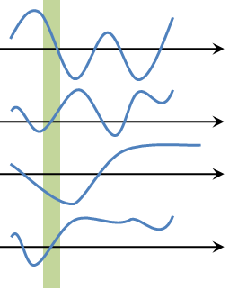
Figure 10.3 shows the sample space of a random process. Each outcome in the sample space is a function. The probability of getting a function is specified by the probability mass or the probability density of the associated random key $\xi$. If you put your hand into the sample space, the sample you pick will be a function that will change with time and is indexed by the random key. From our discussions of joint random variables in Chapter 5, you can think of the function as a vector. When you pull a sample from the sample space, you pull the entire vector and not just an element.

10.1.2Statistical and temporal perspectives

Since a random process is a function indexed by a random key, it is a two-dimensional object. It is a function both of time $t$ and of the random key $\xi$. That's why we use the notation $X(t,\xi)$ to denote a random process. These two axes play different roles, as illustrated in Figure 10.4.

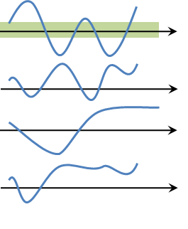
**Figure 10.4.** Temporal and statistical perspectives of a random process. For the temporal perspective (which we call the horizontal perspective), we fix the random key $\xi$ and look at the function in time. For the statistical perspective (which we call the vertical perspective), we fix the time and look at the function at different random keys.

Temporal perspective: Let us fix the random key at $\xi = \xi_0$. This gives us a function $X(t,\xi_0)$. Since $\xi$ is already fixed at $\xi_0$, we are looking at a particular realization drawn from the sample space. This realization is expressed as a function $X(t,\xi_0)$, which is just a deterministic function that evolves over time. There is no randomness associated with it. This is analogous to a random variable. While $X$ itself is a random variable, by fixing the random key $\xi = \xi_0$, $X(\xi_0)$ is just a real number. For random processes, $X(t,\xi_0)$ now becomes a function.

Since $X(t,\xi_0)$ is a function that evolves over time, we view it along the horizontal axis. For example, we can study the sequence

X(t_1,\xi_0), X(t_2,\xi_0), \ldots, X(t_K,\xi_0),

where $t_1,\ldots,t_K$ are the time indices of the function. This sequence is deterministic and is just a sequence of numbers, although the numbers evolve as $t$ changes.

Statistical perspective: The other perspective, which could be slightly more abstract, is the statistical perspective. Let us fix the time at $t = t_0$. The random key $\xi$ can take any state defined in the sample space. So if the sample space contains $\{\xi_1,\ldots,\xi_N\}$, the sequence $\{X(t_0,\xi_1), \ldots, X(t_0,\xi_N)\}$ is a sequence of random variables, because the $\xi$'s can go from one state to another state.

A good way to visualize the statistical perspective is the vertical perspective in which we write the sequence as a vertical column of random variables:

\begin{array}{c} X(t_0,\xi_1) \\ X(t_0,\xi_2) \\ \vdots \\ X(t_0,\xi_N) \end{array}

That is, if you fix the time at $t = t_0$, you are getting a sequence of random variables. The probability of getting a particular value $X(t_0)$ depends on which random state you land on.

Why do we bother to differentiate the temporal perspective and the statistical perspective? The reason is that the operations associated with the two are different, even if sometimes they give you the same result. For example, if we take the temporal average of the random process, we get a number:

\overline{X}(\xi) = \frac{1}{T}\int_0^T X(t,\xi)\;dt.

We call this the “temporal average” because we have integrated the function over time. The resulting value will not change with time. However, $\overline{X}(\xi)$ depends on the random key you provide. If you pick a different random realization, $\overline{X}(\xi)$ will take a different value. So the temporal average is a random variable.

On the other hand, if we take the statistical average of the random process, we get

\E[X(t)] = \int_{\Omega} X(t,\xi) \;p(\xi) \;d\xi,

where $p(\xi)$ is the PDF of the random key $\xi$. We call this the statistical average because we have taken the expectation over all possible random keys. The resulting object $\E[X(t)]$ is deterministic but a function of time.

No matter how you look at the temporal average or the statistical average, they are different with the following exception: that $\overline{X}(\xi) = \text{const}$ and $\E[X(t)] = \text{const}$, for example, $\overline{X}(\xi) = \E[X(t)] = 0$. This happens only for some special (and useful) random processes known as ergodic processes that allow us to approximate the statistical average using the temporal average, with some guarantees derived from the law of large numbers. We will return to this point later.

Example 10.3

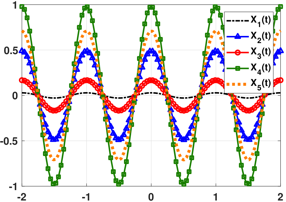
Let $A\sim$Uniform$[0,1]$. Define

X(t,\xi)=A(\xi)\cos(2\pi t).

In this example, the magnitude $A(\xi)$ is a random variable depending on the random key $\xi$. For example if we draw $\xi_1$, perhaps we will get a value $A(\xi_1)=0.5$. Then $X(t,\xi_1)=0.5 \cos(2\pi t)$. To take another example, if we draw $\xi_2$, we may get $A(\xi_2)=1$. Then $X(t,\xi_2)=1 \cos(2\pi t)$. Figure 10.5 shows a few random realizations of the cosines. We can look at $X(t,\xi)$ from the statistical and the temporal views.

**Figure 10.5.** Five different realizations of the random process $X(t) = A\cos(2\pi t)$.

sep0ex
Statistical View: Fix $t$ (for example $t=10$). In this case, we have
$\begin{aligned} X(t,\xi) &=A(\xi)\cos(2 \pi (10))\\ &=A(\xi)\cos(20 \pi), \end{aligned}$
which is a random variable because $\cos(20 \pi)$ is a constant. The randomness of $X$ comes from the fact that $A(\xi)\sim$ Uniform$[0,1]$.
Temporal View: Fix $\xi$ (for example $A(\xi) = 0.7$). In this case, we have $$X(t,\xi)=0.7\cos(2 \pi t),$$ which is a deterministic function of $t$.

Example 10.4

Let $A$ be a discrete random variable with a PMF

\Pb(A=+1)=\frac{1}{2} \;\; \mbox{and} \;\; \Pb(A=-1)=\frac{1}{2}.

We define the function $X[n,\xi]=A(\xi)(-1)^n$. In this example, $A$ can only take two states. If $A=+1$, then $X[n,\xi]=(-1)^n$. If $A=-1$, then $X[n,\xi]=(-1)^{n+1}$.

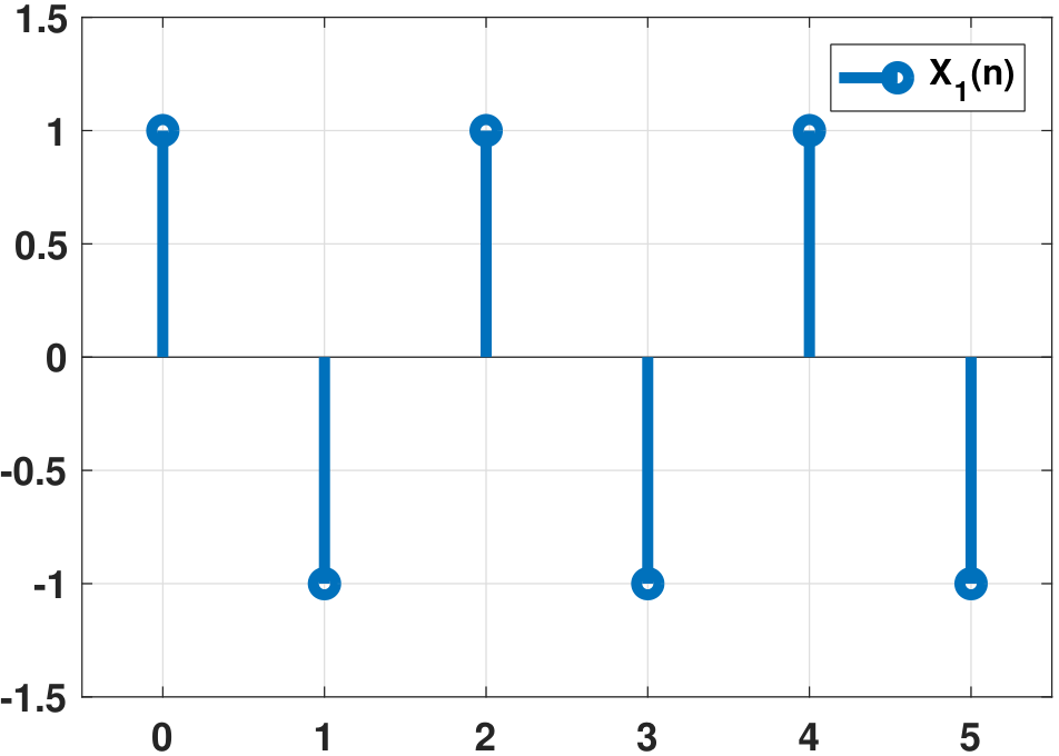
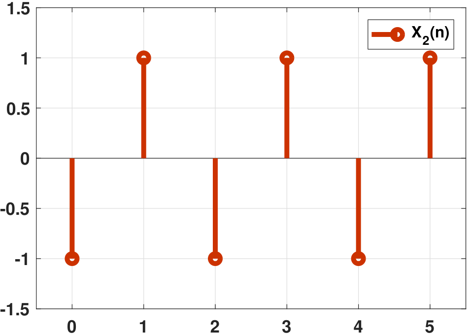
**Figure 10.6.** Realizations of the random process $X[n] = A(-1)^n$.

The graphical illustration of this example is shown in Figure 10.6. Again, we can look at $X[n,\xi]$ from two views.

sep0ex
Statistical View: Fix $n$, say $n = 10$. Then, $$X(\xi) = \begin{cases} (-1)^{10} = 1, &\quad \mbox{with prob}\; 1/2,\\ (-1)^{11} = -1,&\quad \mbox{with prob}\; 1/2, \end{cases}$$ which is a Bernoulli random variable.
Temporal View: Fix $\xi$. Then, $$X[n] = \begin{cases} (-1)^n, &\quad \mbox{if}\;\; A=+1, \\ (-1)^{n+1}, &\quad \mbox{if}\;\; A=-1, \end{cases}$$ which is a time series.

In this example, we see that the sample space of $X[n,\xi]$ consists of only two functions with probabilities

\begin{aligned} &\Pb(X[n]=(-1)^n)=\frac{1}{2}, \\ &\Pb(X[n]=(-1)^{n+1})=\frac{1}{2}, \end{aligned}

Therefore, if there is a sequence outside the sample space, e.g.,

\Pb\left(X[n]=\left[\begin{array}{ccccccc} 1 & 1 & 1 & -1 & 1 & -1 & \cdots \end{array}\right]\right)=0

then the probability of obtaining that sequence is 0.

What do we mean by statistical average and temporal average?

sep0ex
Statistical average: Take the expectation of $X(t,\xi)$ over $\xi$. This is the vertical average.
Temporal average: Take the expectation of $X(t,\xi)$ over $t$. This is the horizontal average.
In general, statistical average $\not=$ temporal average.