Principles of Regression
We start by recalling our discussion in the introduction. The purpose of regression can be summarized in a simple statement:
Given the data points \((x_1,y_1),\ldots,(x_N,y_N)\), find the parameter \(\vtheta\) of a function \(g_{\vtheta}(\cdot)\) such that the training loss is minimized:
where \(\calL(\cdot,\cdot)\) is the loss between a pair of true observation \(y_n\) and the prediction \(g_{\vtheta}(x_n)\).
When the context makes it clear, we will drop the subscript \(\vtheta\) in \(g_{\vtheta}(\cdot)\) with the understanding that the function \(g(\cdot)\) is parameterized by \(\vtheta\).
As you can see, regression finds a function \(g(\cdot)\) that best approximates the input-output relationship between \(x_n\) and \(y_n\). There are two choices we need to make when formulating a regression problem:
- sep0ex
- Function \(g(\cdot)\): What is the family of functions we want to use? This could be a line, a polynomial, or a set of basis functions. If it is a polynomial, what is its order? We need to make all of these decisions before running the regression. A poor choice of function family can lead to a poor regression result.
- Loss “\(\calL(\cdot,\cdot)\)”: How do we measure the closeness between \(y_n\) and \(g(x_n)\)? Are we measuring in terms of the squared error \((y_n-g(x_n))^2\), or the absolute difference \(|y_n-g(x_n)|\), or something else? Again, a poor choice of distance function can create a false sense of closeness because you might be optimizing for a wrong objective.
Before we delve into the details, we need to discuss briefly the connection between regression and probability. A regression problem can be solved without knowing probability, so why is regression discussed in a book on probability?
This question is related to how much we know about the statistical model and what kind of optimality we are seeking. A full answer requires some understanding of maximum likelihood estimation and maximum a posteriori estimation, which will be explained in Chapter 8. As a quick preview of our results, we summarize the key ideas below:
- sep0ex
- If you know the statistical relationship between \(x_n\) and \(y_n\), then we can construct a regression problem that maximizes the likelihood of the underlying distribution. Such regression solution is optimal with respect to the likelihood.
- We can construct a regression problem that can minimize the expectation of the squared error. This regression solution is mean-squared optimal.
- If you are a Bayesian and you know the prior distribution of \(x_n\), then we can construct a regression problem that maximizes the posterior distribution. The solution to this regression problem is Bayesian optimal.
- If you know nothing about the statistics of \(x_n\) and \(y_n\), you can still run the regression and get something, and this “something” can be very useful. However, you cannot claim statistical optimality of this “something”.
See Chapter 8 for additional discussion.
It is important to understand that a regression problem is at the intersection of optimization and statistics. The need for optimization is clear because we need to minimize the error. The statistical need is to generalize to unknown data. If there is no statistical relationship between \(x_n\) and \(y_n\) (for all \(n\)), whatever model we obtain from the regression will only work for the \(N\) training samples. The model will not generalize because knowing \(x_n\) will not help us know \(y_n\). In other words, if there is no statistical relationship between \(x_n\) and \(y_n\), you can fit perfectly to the training data but you will fail miserably to fit the testing data.
7.1.1Intuition: How to fit a straight line?
In this subsection we want to give you the basic idea of how regression is formulated. To keep things simple, we will discuss how to fit data using a straight line.
Consider a collection of data points \(\calD = \{(x_1,y_1),\ldots,(x_N,y_N)\}\), where \(x_n\)'s are the inputs and \(y_n\)'s are the observations, for example, in the table below.
| \(n\) | \(x_n\) | \(y_n\) |
| 1 | 0.6700 | 3.0237 |
| 2 | 0.3474 | 2.3937 |
| 3 | 0.6695 | 3.5548 |
| \(N-1\) | 0.2953 | 2.6396 |
| \(N\) | 0.6804 | 3.2536 |
Let us consider the linear regression problem. The goal of linear regression is to find the straight line that best fits the datasets. All straight lines on a 2D graph are plots of the equation
where \(a\) is the slope of the line and \(b\) is the \(y\)-intercept of the line. We denote this line by \(g(\cdot)\). Note that this function \(g\) is characterized by two parameters \((a,b)\) because once \((a,b)\) are known the line is determined. If we change \((a,b)\), the line will change as well. Therefore, by finding the best line we are essentially searching for the best \((a,b)\) such that the training error is minimized.
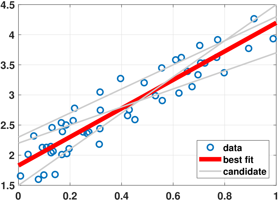
The pictorial meaning of linear regression can easily be seen in Figure 7.1, which shows \(N = 50\) data points according to some latent distributions. Given these 50 data points, we construct several possible candidates for the regression model. These candidates are characterized by the parameters \((a,b)\). For example, the parameters \((a,b) = (1,2)\) and \((a,b) = (-2,3)\) represent two different straight lines in the candidate pool. The goal of the regression is to find the best line from these candidates. Note that since we limit ourselves to straight lines, the candidate set will not include polynomials or trigonometric functions. These functions are outside the family we are considering.
Given these candidate functions, we need to measure the training loss. This can be defined in multiple ways, such as
- sep0ex
- Sum-squared loss \(\calE_{\text{train}}(\vtheta) = \sum_{n=1}^N (y_n - g(x_n))^2\).
- Sum-absolute loss \(\calE_{\text{train}}(\vtheta) = \sum_{n=1}^N |y_n - g(x_n)|\).
- Cross-entropy loss \(\calE_{\text{train}}(\vtheta) = -\sum_{n=1}^N\left( y_n \log g(x_n) + (1-y_n)\log(1-g(x_n))\right)\).
- Perceptual loss \(\calE_{\text{train}}(\vtheta) = \sum_{n=1}^N \max(-y_n g(x_n),0)\), when \(y_n\) and \(g(x_n)\) are binary taking values \(\pm 1\). This is a reasonable training error because if \(y_n\) matches with \(g(x_n)\), then \(y_n g(x_n) = 1\) and so \(\max(-y_n g(x_n),0) = 0\). But if \(y_n\) does not match with \(g(x_n)\), then \(y_n g(x_n) = -1\) and hence \(\max(-y_n g(x_n),0) = 1\). Thus, the loss captures the sum of all the mismatched pairs.
Choosing the loss function is problem-specific. It is also where probability enters the picture because, without any knowledge about the distributions of \(x_n\) and \(y_n\), there is no way to choose the best training loss. You can still pick one, as we will do, but it will not be granted any probabilistic guarantees.
Among these possible choices of the training error, we are going to focus on the sum-squared loss because it is convex and differentiable. This makes the computation easy, since we can run any textbook optimization algorithm. The regression problem under the sum-squared loss is:
In this equation, the symbol “\(\text{argmin}\)” means “argument minimize”, which returns the argument that minimizes the cost function on the right. The interpretation of the equation is that we seek the \((a,b)\) that minimize the sum \(\sum_{n=1}^N (y_n - (ax_n+b))^2\). Since we are minimizing the squared error, this linear regression problem is also known as the least squares fitting problem. The idea is summarized in the following box.
- sep0ex
- Find a line \(g(x) = ax+b\) that best fits the training data \(\{(x_n,y_n)\}_{n=1}^N\).
The optimality criterion is to minimize the squared error
$$\calE_{\text{train}}(\vtheta) = \sum_{n=1}^N \bigg(y_n - g(x_n)\bigg)^2,$$where \(\vtheta = (a,b)\) is the model parameter.
- There exist other optimality criteria. Squared error is convex and differentiable.
7.1.2Solving the linear regression problem
Let's consider how to solve the linear regression problem given by Eq. (7.2). The problem is the following:
As with any two-dimensional optimization problem, the optimal point \((\ahat,\bhat)\) should have a zero gradient, meaning that
This should be familiar to you, even if you have only learned basic calculus. This pair of equations says that, at a minimum point, the directional slopes should be zero no matter which direction you are looking at.
The derivative with respect to \(a\) is
Similarly, the derivative with respect to \(b\) is
Setting these two equations to zero, we have that
Rearranging the terms, the pair can be equivalently written as
Therefore, if we can solve this system of linear equations, we will have the linear regression solution.
Remark. It is easy to see that the solution achieves the minimum instead of the maximum, since the second-order derivatives are positive:
The following theorem summarizes this intermediate result.
The solution of the problem Eq. (7.4)
satisfies the equation
Matrix-vector form of linear regression
The regression can be written as
With \(\mX\), \(\vy\), \(\vtheta\) and \(\ve\), we can write the linear regression problem compactly as
Therefore, the training loss \(\calE_{\text{train}}(\vtheta)\) can be defined as
Now, taking the gradient with respect to \(\vtheta\) yields (This is a basic vector calculus result. For details, you may consult standard texts such as the University of Waterloo's matrix cookbook. https://www.math.uwaterloo.ca/ hwolkowi/matrixcookbook.pdf)
Equating this to zero, we obtain
Eq. (7.6) is called the normal equation.
The normal equation is a convenient way of constructing the system of linear equations. Using the 2-by-2 system shown in Eq. (7.5) as an example, we note that
Therefore, as long as you can construct the \(\mX\) matrix, forming the 2-by-2 system in Eq. (7.5) is straightforward: start with \(\vy = \mX\vtheta\) and then multiply both sides by the matrix transpose \(\mX^T\). The resulting system is what you need. There is nothing to memorize.
Running linear regression on a computer
On a computer, solving the linear regression for a line is straightforward. Let us look at the MATLAB code first.
% MATLAB code to fit data points using a straight line
    N = 50;
    x = rand(N,1)*1;
    a = 2.5;                         % true parameter
    b = 1.3;                         % true parameter
    y = a*x + b + 0.2*rand(size(x)); % Synthesize training data

    X    = [x(:) ones(N,1)];         % construct the X matrix
    theta = X\y(:);                  % solve y = X theta

    t    = linspace(0, 1, 200);      % interpolate and plot
    yhat = theta(1)*t + theta(2);
    plot(x,y,'o','LineWidth',2); hold on;
    plot(t,yhat,'r','LineWidth',4);
In this piece of MATLAB code, we need to define the data matrix \(\mX\). Here, x(:) is the column vector that stores all the values \((x_1,\ldots,x_N)\). The all-one vector ones(N,1) is the second column in our \(\mX\) matrix. The command X\y(:) is equivalent to solving the normal equation
The last few lines are used to plot the predicted curve. Note that theta(1) and theta(2) are the entries of the solution \(\vtheta\). The result of this program is exactly the plot shown in Figure 7.1 above.
In Python, the program is quite similar. The command we use to solve the inversion is np.linalg.lstsq.
# Python code to fit data points using a straight line
    import numpy as np
    import matplotlib.pyplot as plt

    N = 50
    x = np.random.rand(N)
    a = 2.5                                 # true parameter
    b = 1.3                                 # true parameter
    y = a*x + b + 0.2*np.random.randn(N)    # Synthesize training data

    X = np.column_stack((x, np.ones(N)))    # construct the X matrix
    theta = np.linalg.lstsq(X, y, rcond=None)[0] # solve y = X theta

    t = np.linspace(0,1,200)                # interpolate and plot
    yhat = theta[0]*t + theta[1]
    plt.plot(x,y,'o')
plt.plot(t,yhat,'r',linewidth=4)7.1.3Extension: Beyond a straight line
Regression is a powerful technique. Although we have discussed its usefulness for fitting straight lines, the same concept can fit other curves.
To generalize the regression formulation, we consider a \(d\)-dimensional regression coefficient vector \(\vtheta = [\theta_0,\ldots,\theta_{d-1}]^T \in \R^d\) and a general linear model
Here, the mappings \(\{\phi_p(\cdot)\}_{p=0}^{d-1}\) can be considered as a nonlinear transformation that takes the input \(x_n\) and maps it to another value. For example, \(\phi_p(\cdot) = (\cdot)^p\) will map an input \(x\) to a \(p\)th power \(x^p\).
We can now write the system of linear equations as
Let us look at some examples.
(Quadratic fitting) Consider the linear regression problem using a quadratic equation:
Express this equation in matrix-vector form.
The matrix-vector expression is
This is again in the form of \(\vy = \mX\vtheta + \ve\).
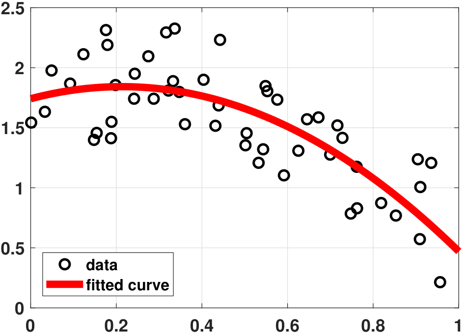
The MATLAB and Python programs for Example 7.1 are shown below. A numerical example is illustrated in Figure 7.2.
% MATLAB code to fit data using a quadratic equation
    N = 50;
    x = rand(N,1)*1;
    a = -2.5;
    b = 1.3;
    c = 1.2;
    y = a*x.^2 + b*x + c + 1*rand(size(x));

    N    = length(x);
    X    = [ones(N,1) x(:) x(:).^2];
    beta = X\y(:);
    t    = linspace(0, 1, 200);
    yhat = theta(3)*t.^2 + theta(2)*t + theta(1);
    plot(x,y,   'o','LineWidth',2); hold on;
plot(t,yhat,'r','LineWidth',6);# Python code to fit data using a quadratic equation
import numpy as np
import matplotlib.pyplot as plt
N = 50
x = np.random.rand(N)
a = -2.5
b = 1.3
c = 1.2
y = a*x**2 + b*x + c + 0.2*np.random.randn(N)
X = np.column_stack((np.ones(N), x, x**2))
theta = np.linalg.lstsq(X, y, rcond=None)[0]
t = np.linspace(0,1,200)
yhat = theta[0] + theta[1]*t + theta[2]*t**2
plt.plot(x,y,'o')
plt.plot(t,yhat,'r',linewidth=4)The generalization to polynomials of arbitrary order is to replace the model with
where \(p = 0,1,\ldots,{d-1}\) represent the orders of the polynomials and \(\theta_0,\ldots,\theta_{d-1}\) are the regression coefficients. In this case, the matrix system is
which again is in the form of \(\vy = \mX\vtheta + \ve\).
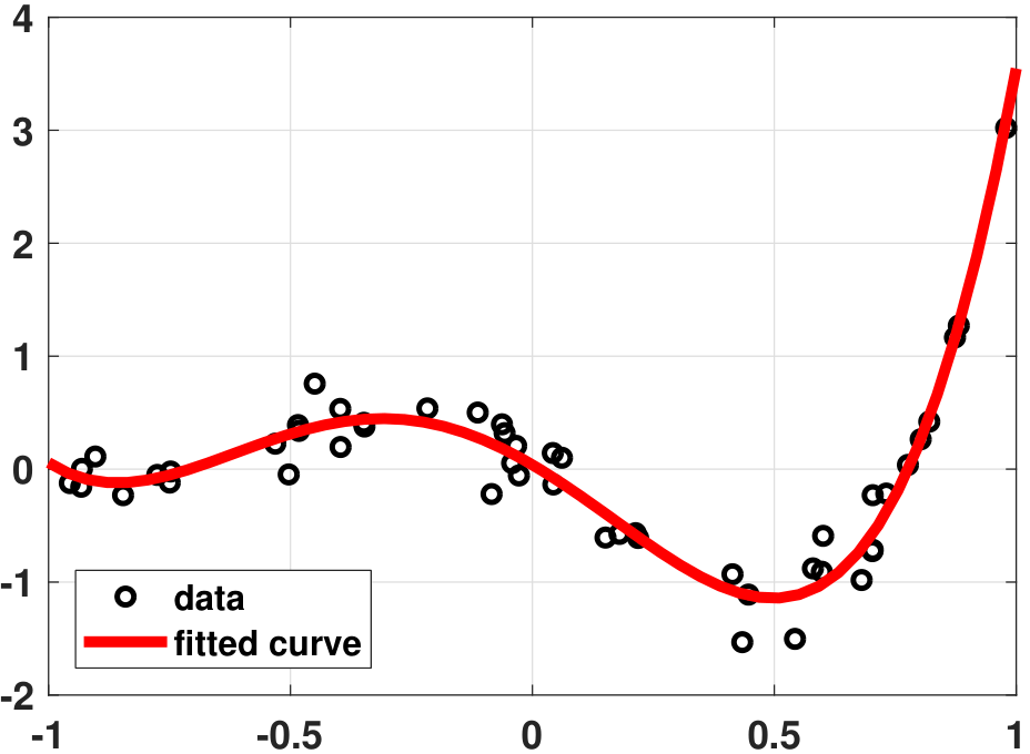
(Legendre polynomial fitting) Let \(\{L_p(\cdot)\}_{p=0}^{d-1}\) be a set of Legendre polynomials (see discussions below), and consider the linear regression problem using
Express this equation in matrix-vector form.
The matrix-vector expression is
Legendre polynomials are orthogonal polynomials. In conventional polynomials, the functions \(\{x,x^2,x^3,\ldots,x^p\}\) are not orthogonal. As we increase \(p\), the set \(\{x,x^2,x^3,\ldots,x^p\}\) will have redundancy, which will eventually result in the matrix \(\mX\) being noninvertible.
The \(p\)th-order Legendre polynomial is denoted by \(L_p(x)\). Using the Legendre polynomials as the building block of the regression problem, the model is expressed as
where \(L_0(\cdot)\), \(L_1(\cdot)\) and \(L_2(\cdot)\) are the Legendre polynomials of order 0, 1 and 2, respectively. As an example, the first few leading Legendre polynomials are
The order of the Legendre polynomials is always the same as that of the ordinary polynomials. The shapes of these polynomials are shown in Figure 7.3(a).
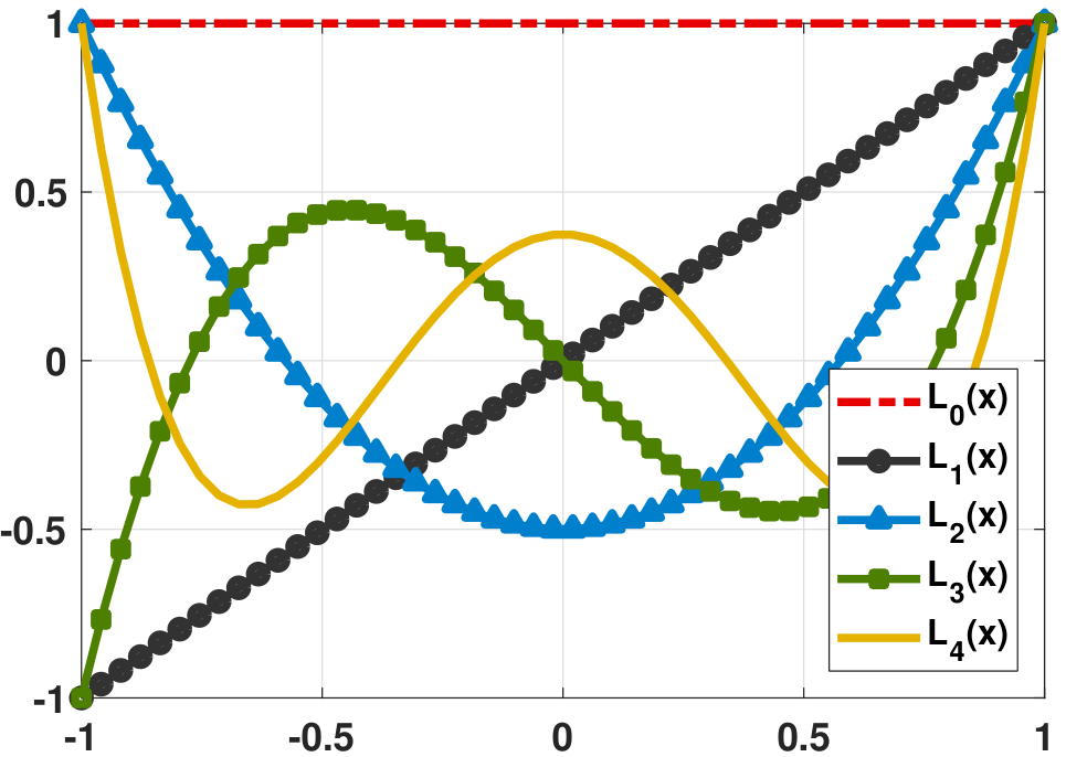
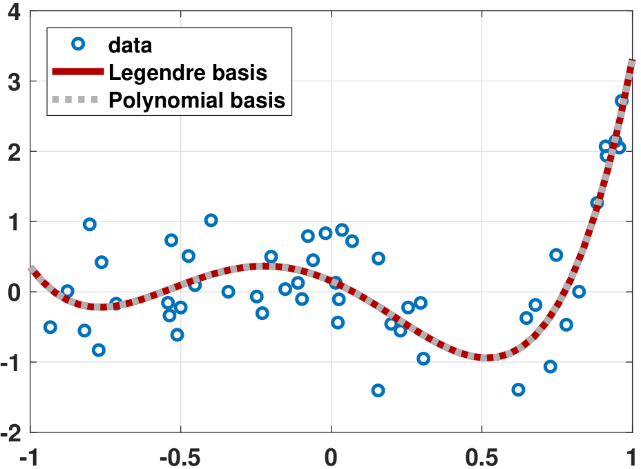
Figure 7.3(b) demonstrates a fitting problem using the Legendre polynomials. You can see that the fitting is just as good as that of the ordinary polynomials (which should be the case). However, if we compare the coefficients, we observe that the magnitude of the Legendre coefficients is smaller (see Table 7.2). In general, as the order of polynomials increases and the noise grows, the ordinary polynomials will become increasingly difficult to fit the data.
| \(\theta_4\) | \(\theta_3\) | \(\theta_2\) | \(\theta_1\) | \(\theta_0\) | |
| Ordinary polynomials | 5.3061 | 3.3519 | \(-\)3.6285 | \(-\)1.8729 | 0.1540 |
| Legendre polynomials | 1.2128 | 1.3408 | 0.6131 | 0.1382 | 0.0057 |
Calling Legendre polynomials for regression is not difficult in MATLAB and Python. Specifically, one can call legendreP in MATLAB and scipy.special.eval_legendre in Python.
% MATLAB code to fit data using Legendre polynomials
    N = 50;
    x = 1*(rand(N,1)*2-1);
    a = [-0.001 0.01 +0.55 1.5 1.2];
    y = a(1)*legendreP(0,x) + a(2)*legendreP(1,x) + ...
      + a(3)*legendreP(2,x) + a(4)*legendreP(3,x) + ...
      + a(5)*legendreP(4,x) + 0.5*randn(N,1);

    X = [legendreP(0,x(:)) legendreP(1,x(:)) ...
         legendreP(2,x(:)) legendreP(3,x(:)) ...
         legendreP(4,x(:))];
    beta = X\y(:);

    t    = linspace(-1, 1, 200);
    yhat = beta(1)*legendreP(0,t) + beta(2)*legendreP(1,t) + ...
         + beta(3)*legendreP(2,t) + beta(4)*legendreP(3,t) + ...
         + beta(5)*legendreP(4,t);
    plot(x,y,'ko','LineWidth',2,'MarkerSize',10); hold on;
plot(t,yhat,'LineWidth',6,'Color',[0.9 0 0]);import numpy as np
import matplotlib.pyplot as plt
from scipy.special import eval_legendre
N = 50
x = np.linspace(-1,1,N)
a = np.array([-0.001, 0.01, 0.55, 1.5, 1.2])
y = a[0]*eval_legendre(0,x) + a[1]*eval_legendre(1,x) + \
a[2]*eval_legendre(2,x) + a[3]*eval_legendre(3,x) + \
a[4]*eval_legendre(4,x) + 0.2*np.random.randn(N)
X = np.column_stack((eval_legendre(0,x), eval_legendre(1,x), \
eval_legendre(2,x), eval_legendre(3,x), \
eval_legendre(4,x)))
theta = np.linalg.lstsq(X, y, rcond=None)[0]
t = np.linspace(-1, 1, 50);
yhat = theta[0]*eval_legendre(0,t) + theta[1]*eval_legendre(1,t) + \
theta[2]*eval_legendre(2,t) + theta[3]*eval_legendre(3,t) + \
theta[4]*eval_legendre(4,t)
plt.plot(x,y,'o',markersize=12)
plt.plot(t,yhat, linewidth=8)
plt.show()The idea of fitting a set of data using the Legendre polynomials belongs to the larger family of basis functions. In general, we can use a set of basis functions to model the data:
where \(\{\phi_p(x)\}_{p=0}^{d-1}\) are the basis functions and \(\{\theta_p\}_{p=0}^{d-1}\) are the regression coefficients. The constant \(\theta_0\) is often called the bias of the regression.
Choice of the \(\phi_p(x)\) can be extremely broad. One can choose the ordinary polynomials \(\phi_p(x) = x^p\) or the Legendre polynomial \(\phi_p(x) = L_p(x)\). Other choices are also available:
- Fourier basis: \(\phi_p(x) = e^{j \omega_p x}\), where \(\omega_p\) is the \(p\)th carrier frequency.
- Sinusoid basis: \(\phi_p(x) = \sin(\omega_p x)\), which is the same as the Fourier basis but taking the imaginary part.
- Gaussian basis: \(\phi_p(x) = \frac{1}{\sqrt{2\pi \sigma_p^2}} \exp\left\{-\frac{(x-\mu_p)^2}{2\sigma_p^2}\right\}\), where \((\mu_p,\sigma_p)\) are the model parameters.
Evidently, by choosing different basis functions we have different ways to fit the data. There is no definitive answer as to which functions are better. Statistical techniques such as model selections are available, but experience will tell you to align with one and not the other. It is frequently more useful to have some domain knowledge rather than resorting to various computational techniques.
- sep0ex
Construct this equation:
$$\underset{\vy}{\underbrace{ \begin{bmatrix} y_1\\ y_2\\ \vdots \\ y_N \end{bmatrix}}} = \underset{\mX}{\underbrace{ \begin{bmatrix} \phi_0(x_1) & \phi_1(x_1) & \cdots & \phi_{d-1}(x_1)\\ \phi_0(x_2) & \phi_1(x_2) & \cdots & \phi_{d-1}(x_2)\\ \vdots & \cdots & \vdots & \vdots \\ \phi_0(x_N) & \phi_1(x_N) & \cdots & \phi_{d-1}(x_N)\\ \end{bmatrix}}} \underset{\vtheta}{\underbrace{ \begin{bmatrix} \theta_0\\ \theta_1\\ \vdots\\ \theta_{d-1} \end{bmatrix}}} + \underset{\ve}{\underbrace{ \begin{bmatrix} e_1\\ e_2\\ \vdots\\ e_N \end{bmatrix}}},$$- The functions \(\phi_p(x)\) are the basis functions, e.g., \(\phi_p(x) = x^p\) for ordinary polynomials.
- You can replace the polynomials with the Legendre polynomials.
- You can also replace the polynomials with other basis functions.
Solve for \(\vtheta\) by
$$\vthetahat = \argmin{\vtheta} \;\; \|\vy - \mX\vtheta\|^2.$$
(Autoregressive model) Consider a two-tap autoregressive model:
where we assume \(y_0 = y_{-1} = 0\). Express this equation in the matrix-vector form.
The matrix-vector form of the equation is
In general, we can append more previous samples to predict the future. The general expression is
where \(\ell = 1,2,\ldots,L\) denote the previous \(L\) samples of the data and \(\{\theta_1,\ldots,\theta_L\}\) are the regression coefficients. If we do this we see that the matrix expression is
Observe the pattern associated with this matrix \(\mX\). Each column is a one-entry shifted version of the previous column. This matrix is called a Toeplitz matrix.
The MATLAB (and Python) code for calling and using the Toeplitz matrix is shown below.
% MATLAB code for auto-regressive model
    N = 500;
    y = cumsum(0.2*randn(N,1)) + 0.05*randn(N,1);   % generate data

    L = 100;                                        % use previous 100 samples
    c = [0; y(1:400-1)];
    r = zeros(1,L);
    X = toeplitz(c,r);                              % Toeplitz matrix
    theta = X\y(1:400);                             % solve y = X theta
    yhat = X*theta;                                 % prediction
    plot(y(1:400),   'ko','LineWidth',2);hold on;
plot(yhat(1:400),'r','LineWidth',4);# Python code for auto-regressive model
import numpy as np
import matplotlib.pyplot as plt
from scipy.linalg import toeplitz
N = 500
y = np.cumsum(0.2*np.random.randn(N)) + 0.05*np.random.randn(N)
L = 100
c = np.hstack((0, y[0:400-1]))
r = np.zeros(L)
X = toeplitz(c,r)
theta = np.linalg.lstsq(X, y[0:400], rcond=None)[0]
yhat = np.dot(X, theta)
plt.plot(y[0:400], 'o')
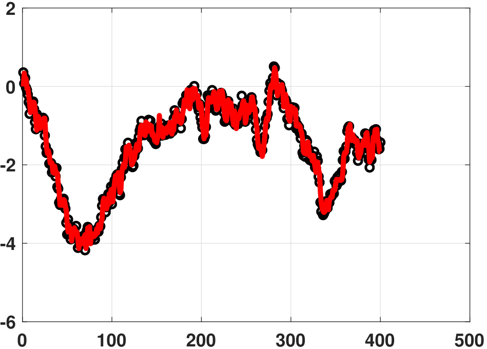
plt.plot(yhat[0:400],linewidth=4)The plots generated by the above programs are shown in Figure 7.4(a). Note that we are doing an interpolation, because we are predicting the values within the training dataset.
We now consider extrapolation. Given the training data, we can find the regression coefficients by solving the above linear equation. This gives us \(\vtheta\). To predict the future samples we need to return to the equation
where \(\yhat_{n-\ell}\) are the previous estimates. For example, if we are given 100 days of stock prices, then predicting the 101st day's price should be based on the \(L\) days before the 101st. A simple for-loop suffices for such a calculation.
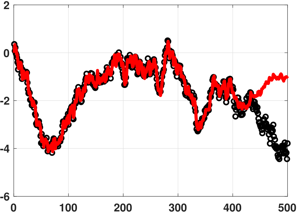
Figure 7.4(b) shows a numerical example of extrapolating data using the autoregressive model. In this experiment we use \(N = 400\) samples to train an autoregressive model of order \(L = 100\). We then predict the data for another 100 data points. As you can see from the figure, the first few samples still look reasonable. However, as time increases, the model starts to lose track of the real trend.
Is there any way we can improve the autoregressive model? A simple way is to increase the memory \(L\) so that we can use a long history to predict the future. This boils down to the long-term running average of the curve, which works well in many cases. However, if the testing data does not follow the same distribution as the training data (which is often the case in the real stock market because unexpected news can change the stock price), then even the long-term average will not be a good forecast. That is why data scientists on Wall Street make so much money: they have advanced mathematical tools for modeling the stock market. Nevertheless, we hope that the autoregressive model provides you with a new perspective for analyzing data.
The summary below highlights the main ideas of the autoregressive model.
- sep0ex
It solves this problem
$$\underset{=\vy}{\underbrace{\begin{bmatrix} y_1\\ y_2\\ y_3\\ \vdots \\ y_N \end{bmatrix}}} = \underset{=\mX}{\underbrace{ \begin{bmatrix} y_0 & y_{-1} & y_{-2} & \cdots & y_{1-L}\\ y_1 & y_0 & y_{-1} & \cdots & y_{2-L}\\ y_2 & y_1 & y_{0} & \cdots & y_{3-L}\\ \vdots & \vdots & \vdots & \vdots & \vdots\\ y_{N-1} & y_{N-2} & y_{N-3} & \vdots & y_{N-L} \end{bmatrix}}} \underset{=\vtheta}{\underbrace{ \begin{bmatrix} \theta_1\\ \theta_2\\ \vdots\\ \theta_L \end{bmatrix} }} + \underset{=\ve}{\underbrace{ \begin{bmatrix} e_1\\ e_2\\ e_3\\ \vdots \\ e_N \end{bmatrix}}}.$$- The number of taps in the past history would affect the memory and hence the long-term forecast.
Solve for \(\vtheta\) by
$$\vthetahat = \argmin{\vtheta \in \R^d} \;\; \|\vy - \mX\vtheta\|^2.$$
7.1.4Overdetermined and underdetermined systems
The sub-section requires knowledge of some concepts in linear algebra that can be found in standard references. (Carl Meyer, Matrix Analysis and Applied Linear Algebra, SIAM, 2000.)
Let us now consider the theoretical properties of the least squares linear regression problem, which is an optimization:
We observe that the objective value of this optimization problem can go to zero if and only if the minimizer \(\vthetahat\) is the solution of the system of linear equations
We emphasize that Problem (eq: ch7 least square main problem) and Problem (eq: ch7 least square main problem 2) are two different problems. Even if we cannot solve Problem (eq: ch7 least square main problem 2), Problem (eq: ch7 least square main problem) is still well defined, but the objective value will not go to zero. This subsection aims to draw the connection between the two problems and discuss the respective solutions. We will start with Problem (eq: ch7 least square main problem 2) by considering two shapes of the matrix \(\mX\).
Overdetermined system
Problem (eq: ch7 least square main problem 2) is called overdetermined if \(\mX \in \R^{N \times d}\) is tall and skinny, i.e., \(N > d\). This happens when you have more rows than columns, or equivalently when you have more equations than unknowns. When \(N > d\), Problem (eq: ch7 least square main problem 2) has a unique solution \(\vthetahat = (\mX^T\mX)^{-1}\mX^T\vy\) if and only if \(\mX^T\mX\) is invertible, or equivalently if and only if the columns of \(\mX\) are linearly independent. A technical description of this is that \(\mX\) has a full rank, denoted by \(\text{rank}(\mX) = d\). When \(\text{rank}(\mX) = d\), Problem (eq: ch7 least square main problem) has a unique global minimizer \(\vthetahat = (\mX^T\mX)^{-1}\mX^T\vy\), which is the same as the unique solution of Problem (eq: ch7 least square main problem 2).
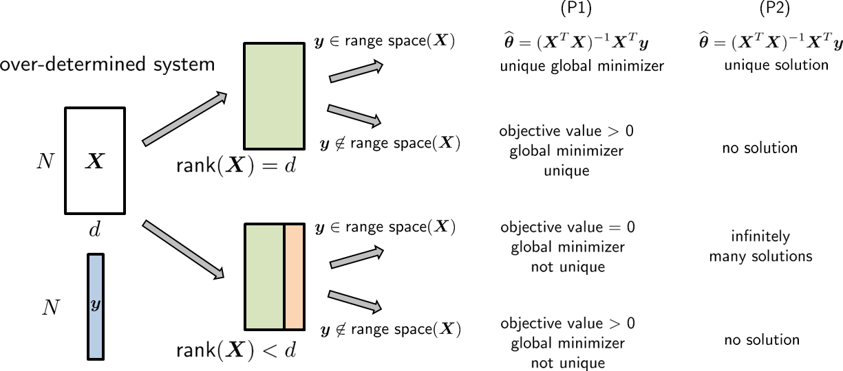
If the columns of \(\mX\) are linearly dependent so that \(\mX^T\mX\) is not invertible, we say that \(\mX\) is rank-deficient (denoted as \(\text{rank}(\mX) < d\)). In this case, Problem (eq: ch7 least square main problem 2) may not have a solution. We say that it may not have a solution because it is still possible to have a solution. It all depends on whether \(\vy\) can be written as a linear combination of the linearly independent columns of \(\mX\).
If yes, we say that \(\vy\) lives in the range space of \(\mX\). The range space of \(\mX\) is defined as the set of vectors \(\{\vz \,|\, \vz = \mX\valpha, \; \text{for some}\; \valpha\}\). If \(\text{rank}(\mX) = d\), all \(\vy\) will live in the range space of \(\mX\). But if \(\text{rank}(\mX) < d\), only some of the \(\vy\) will live in the range space of \(\mX\). When this happens, the matrix \(\mX\) must have a nontrivial null space. The null space of \(\mX\) is defined as the set of vectors \(\{\vz \,|\, \mX\vz = 0\}\). A nontrivial null space will give us infinitely many solutions to Problem (eq: ch7 least square main problem 2). This is because if \(\valpha\) is the solution found in the range space so that \(\vy = \mX\valpha\), then we can pick any \(\vz\) from the null space such that \(\mX\vz = 0\). This will lead to another solution \(\valpha + \vz\) such that \(\mX(\valpha+\vz) = \mX\valpha + 0 = \vy\). Since we have infinitely many choices of such \(\vz\)'s, there will be infinitely many solutions to Problem (eq: ch7 least square main problem 2).
Although there are infinitely many solutions to Problem (eq: ch7 least square main problem 2), all of them are the global minimizers of Problem (eq: ch7 least square main problem). They can make the objective value equal to zero because the equality \(\vy = \mX\vtheta\) holds. However, the solutions to Problem (eq: ch7 least square main problem 2) are not unique since the objective function is convex but not strictly convex.
If \(\vy\) does not live in the range space of \(\mX\), we say that Problem (eq: ch7 least square main problem 2) is incompatible. If a system of linear equations is incompatible, there is no solution. However, even when this happens, we can still solve the optimization Problem (eq: ch7 least square main problem), but the objective value will not reach 0. The minimizer is a global minimizer because the objective function is convex, but the minimizer is not unique.
Underdetermined system
Problem (eq: ch7 least square main problem 2) is called underdetermined if \(\mX\) is fat and short, i.e., \(N < d\). This happens when you have more columns than rows, or equivalently when you have more unknowns than equations. In this case, \(\mX^T\mX\) is not invertible, and so we cannot use \(\vthetahat = (\mX^T\mX)^{-1}\mX^T\vy\) as the solution. However, if \(\text{rank}(\mX) = N\), then any \(\vy\) will live in the range space of \(\mX\). But because \(\mX\) is fat and short, there exists a nontrivial null space. Therefore, Problem (eq: ch7 least square main problem 2) will have infinitely many solutions, attributed to the vectors generated by the null space. For this set of infinitely many solutions, the corresponding Problem (eq: ch7 least square main problem) will have a global minimizer, and the objective value will be zero. However, the minimizer is not unique. This is the first case in Figure 7.6.
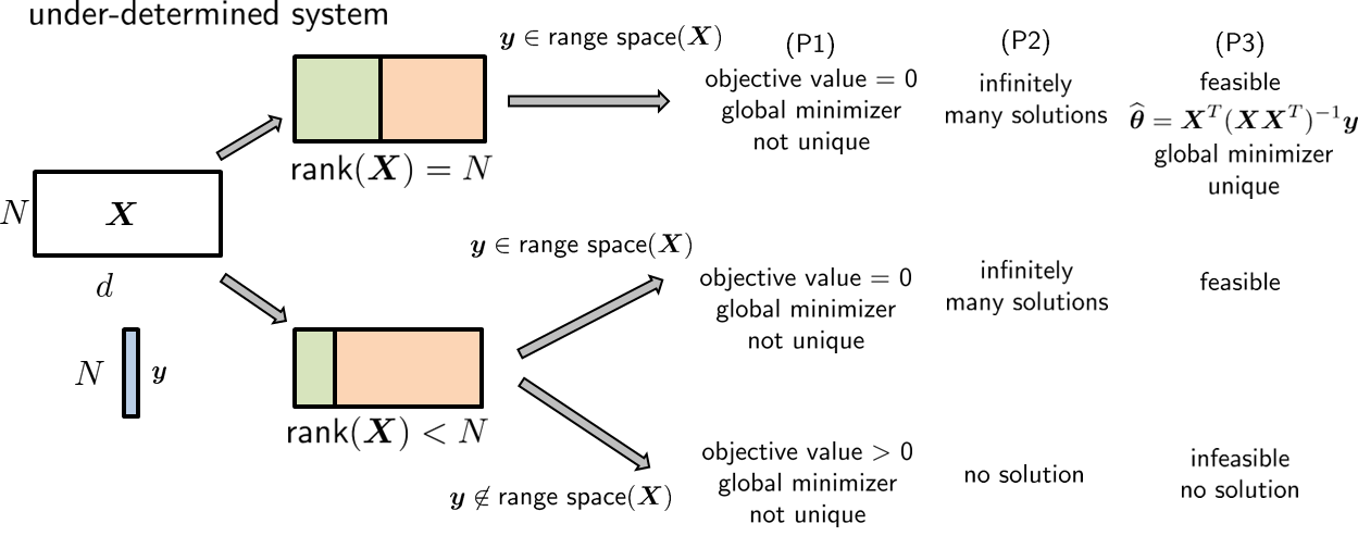
There are two other cases in Figure 7.6, which occur when \(\text{rank}(\mX) < N\):
- sep0ex
- (i) If \(\vy\) is in the range space of \(\mX\), Problem (eq: ch7 least square main problem 2) will have infinitely many solutions. Since Problem (eq: ch7 least square main problem 2) remains feasible, the objective function of Problem (eq: ch7 least square main problem) will go to zero.
- (ii) If \(\vy\) is not in the range space of \(\mX\), the system in Problem (eq: ch7 least square main problem 2) is incompatible and there will be no solution. The objective value of Problem (eq: ch7 least square main problem) will not go to zero.
If an underdetermined system has infinitely many solutions, we need to pick and choose. One of the possible approaches is to consider the optimization
This optimization is different from Problem (eq: ch7 least square main problem), which is an unconstrained optimization. Our goal is to minimize the deviation between \(\mX\vtheta\) and \(\vy\). Problem (eq: ch7 least square alternative problem) is constrained. Since we assume that Problem (eq: ch7 least square main problem 2) has infinitely many solutions, the constraint set \(\vy = \mX\vtheta\) is feasible. Among all the feasible choices, we pick the one that minimizes the squared norm. Therefore, the solution to Problem (eq: ch7 least square alternative problem) is called the minimum-norm least squares. Theorem thm: ch7 under-determined below summarizes the solution. If \(\vy\) does not live in the range space of \(\mX\), then Problem (eq: ch7 least square main problem 2) does not have a solution. Therefore, the constraint in eq: ch7 least square alternative problem is infeasible, and hence the optimization problem does not have a minimizer.
Consider the underdetermined linear regression problem where \(N < d\):
where \(\mX \in \R^{N \times d}\), \(\vtheta \in \R^d\), and \(\vy \in \R^N\). If \(\text{rank}(\mX) = N\), then the linear regression problem will have a unique global minimum
This solution is called the minimum-norm least-squares solution.
Proof. The proof of the theorem requires some knowledge of constrained optimization. Consider the Lagrangian of the problem:
where \(\vlambda\) is called the Lagrange multiplier. The solution of the constrained optimization is the stationary point of the Lagrangian. To find the stationary point, we take the derivatives with respect to \(\vtheta\) and \(\vlambda\). This yields
The first equation gives us \(\vtheta = -\mX^T\vlambda/2\). Substituting it into the second equation, and assuming that \(\text{rank}(\mX) = N\) so that \(\mX\mX^T\) is invertible, we have
which implies that \(\vlambda = -2(\mX\mX^T)^{-1}\vy\). Therefore, \(\vtheta = \mX^T(\mX\mX^T)^{-1}\vy\).
■The end of this subsection. Please join us again.
7.1.5Robust linear regression
This subsection is optional for a first reading of the book.
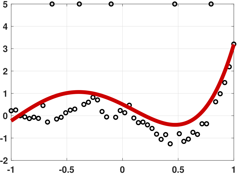
The linear regression we have discussed so far is based on an important criterion, namely the squared error criterion. We chose the squared error as the training loss because it is differentiable and convex. Differentiability allows us to take the derivative and locate the minimum point. Convexity allows us to claim a global minimizer (also unique if the objective function is strictly convex). However, such a nice criterion suffers from a serious drawback: the issue of outliers.
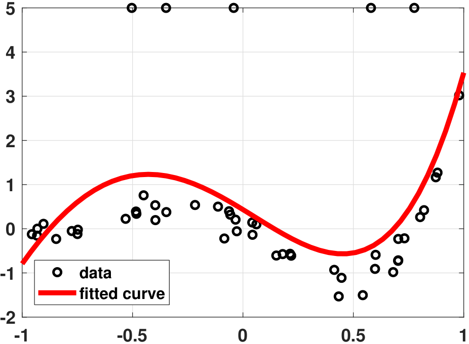
Consider Figure 7.7. In Figure 7.7(a), we show a regression problem for \(N=50\) data points. Our basis functions are the ordinary polynomials in the fourth order. Everything looks fine in the figure. We intervene in the data by randomly altering a few of them so that their values are off. There are only a handful of these outliers. We run the same regression analysis again, but we observe (see Figure 7.7(b)) that our fitted curve has been distorted quite significantly.
This occurs because of the squared error. By the definition of a squared error, our training loss is
Without loss of generality, let us assume that one of these error terms is large because of an outlier. Then the training loss becomes
Here is the daunting fact: If one or a few of these individual error terms are large, the square operation will amplify them. As a result, the error you see is not just redlarge but redlarge\(^2\). Moreover, since we put the squares to the small errors as well, we have blacksmall\(^2\) instead of blacksmall. When you try to weigh the relative significance between the outliers and the normal data points, the outliers suddenly have a very large contribution to the error. Since the goal of linear regression is to minimize the total loss, the presence of the outliers will drive the optimization solution to compensate for the large error.
One possible solution is to replace the squared error by the absolute error, such that
This is a simple modification, but it is very effective. The reason is that the absolute error keeps the bluesmall just as bluesmall, and keeps the redlarge just as redlarge. There is no amplification. Therefore, while the outliers still contribute to the overall loss, their contributions are less prominent. (If you have a lot of strong outliers, even the absolute error will fail. If this happens, you should go back to your data collection process and find out what has gone wrong.)
When we use the absolute error as the training loss, the resulting regression problem is the least absolute deviation regression (or simply the robust regression). The tricky thing about the least absolute deviation is that the training loss is not differentiable. In other words, we cannot take the derivative and find the optimal solution. The good news is that there exists an alternative approach for solving this problem: using linear programming (implemented via the simplex method).
Solving the robust regression problem
Let us focus on the linear model
where \(\vx_n = [\phi_0(x_n),\ldots,\phi_{d-1}(x_n)]^T \in \R^d\) is the \(n\)th input vector for some basis functions \(\{\phi_p\}_{p=0}^{d-1}\), and \(\vtheta = [\theta_0,\ldots,\theta_{d-1}]^T \in \R^d\) is the parameter. Substituting this into the training loss, the optimization problem is
Here is an important trick. The idea is to express the problem as an equivalent problem
There is a small but important difference between this problem and the previous one. In the first problem, there is only one optimization variable \(\vtheta\). In the new problem, we introduce an additional variable \(\vu = [u_1,\ldots,u_N]^T\) and add a constraint \(u_n = |y_n - \vx_n^T\vtheta|\) for \(n = 1,\ldots,N\). We introduce \(\vu\) so that we can have some additional degrees of freedom. At the optimal solution, \(u_n\) must equal \(|y_n - \vx_n^T\vtheta|\), and so the corresponding \(\vtheta\) is the solution of the original problem.
Now we note that \(x = |a|\) is equivalent to \(x \ge a\) and \(x \ge -a\). Therefore, the constraint can be equivalently written as
In other words, we have rewritten the equality constraint as a pair of inequality constraints by removing the absolute signs.
The optimization in Eq. (7.15) is in the form of a standard linear programming problem. A linear programming problem takes the form of
for some vectors \(\vc \in \R^k\), \(\vb \in \R^m\), and matrix \(\mA \in \R^{m \times k}\). Linear programming is a standard optimization problem that you can find in most optimization textbooks. On a computer, if we know \(\vc\), \(\vb\) and \(\mA\), solving the linear programming problem can be done using built-in commands. For MATLAB, the command is linprog. For Python, the command is scipy.optimize.linprog. We will discuss a concrete example shortly.
% MATLAB command for linear programming
x = linprog(c, A, b);# Python command for linear programming
linprog(c, A, b, bounds=(None,None), method="revised simplex")Given Eq. (7.15), the question becomes how to convert it into the standard linear programming format. This requires two steps. The first step uses the objective function:
Therefore, the vector \(\vc\) has \(d\) \(0\)'s followed by \(N\) \(1\)'s.
The second step concerns the constraint. It can be shown that \(u_n \ge -(y_n - \vx_n^T\vtheta)\) is equivalent to \(\vx_n^T\vtheta - u_n \le y_n\). Written in the matrix form, we have
which is equivalent to
where \(\mI \in \R^{N \times N}\) is the identity matrix.
Similarly, the other constraint \(u_n \ge (y_n- \vx_n^T\vtheta)\) is equivalent to \(-\vx_n^T\vtheta - u_n \le -y_n\). Written in the matrix form, we have
which is equivalent to
Putting everything together, we have finally arrived at the linear programming problem
where \(\vzero_d \in \R^d\) is an all-zero vector, and \(\vone_N \in \R^N\) is an all-one vector. It is this problem that solves the robust linear regression.
Let us look at how to implement linear programming to solve the robust regression optimization. As an example, we continue with the polynomial fitting problem in which there are outliers. We choose the ordinary polynomials as the basis functions. To construct the linear programming problem, we need to define the matrix \(\mA\) and the vectors \(\vc\) and \(\vb\) according to the linear programming form. This is done using the following MATLAB program.
% MATLAB code to demonstrate robust regression
    N = 50;
    x = linspace(-1,1,N)';
    a = [-0.001 0.01 0.55 1.5 1.2];
    y = a(1)*legendreP(0,x) + a(2)*legendreP(1,x) + ...
        a(3)*legendreP(2,x) + a(4)*legendreP(3,x) + ...
        a(5)*legendreP(4,x) + 0.2*randn(N,1);
    idx  = [10, 16, 23, 37, 45];
    y(idx) = 5;

    X    = [x(:).^0 x(:).^1 x(:).^2 x(:).^3 x(:).^4];
    A    = [X -eye(N); -X -eye(N)];
    b    = [y(:); -y(:)];
    c    = [zeros(1,5) ones(1,N)]';
    theta = linprog(c, A, b);

    t    = linspace(-1,1,200)';
    yhat = theta(1) + theta(2)*t(:) + ...
           theta(3)*t(:).^2 + theta(4)*t(:).^3 + ...
           theta(5)*t(:).^4;
    plot(x,y,   'ko','LineWidth',2); hold on;
    plot(t,yhat,'r','LineWidth',4);
In this set of commands, the basis vectors are defined as \(\vx_n^T = [\phi_0(x_n),\ldots,\phi_4(x_n)]^T\), for \(n = 1,\ldots,N\). The matrix \(\mI\) is constructed by using the command eye(N), which constructs the identity matrix of size \(N \times N\). The rest of the commands are self-explanatory. Note that the solution to the linear programming problem consists of both \(\vtheta\) and \(\vu\). To squeeze \(\vtheta\) we need to locate the first \(d\) entries. The remainder is \(\vu\).
Commands for Python are similar, although we need to call np.hstack and np.vstack to construct the matrices and vectors. The main routine is linprog in the scipy.optimize library. Note that for this particular example, the bounds are bounds=(None,None), or otherwise Python will search in the positive quadrant.
# Python code to demonstrate robust regression
import numpy as np
import matplotlib.pyplot as plt
from scipy.special import eval_legendre
from scipy.optimize import linprog
N = 50
x = np.linspace(-1,1,N)
a = np.array([-0.001, 0.01, 0.55, 1.5, 1.2])
y = a[0]*eval_legendre(0,x) + a[1]*eval_legendre(1,x) + \
a[2]*eval_legendre(2,x) + a[3]*eval_legendre(3,x) + \
a[4]*eval_legendre(4,x) + 0.2*np.random.randn(N)
idx = [10,16,23,37,45]
y[idx] = 5
X = np.column_stack((np.ones(N), x, x**2, x**3, x**4))
A = np.vstack((np.hstack((X, -np.eye(N))), np.hstack((-X, -np.eye(N)))))
b = np.hstack((y,-y))
c = np.hstack((np.zeros(5), np.ones(N)))
res = linprog(c, A, b, bounds=(None,None), method="revised simplex")
theta = res.x
t = np.linspace(-1,1,200)
yhat = theta[0]*np.ones(200) + theta[1]*t + theta[2]*t**2 + \
theta[3]*t**3 + theta[4]*t**4
plt.plot(x,y,'o',markersize=12)
plt.plot(t,yhat, linewidth=8)
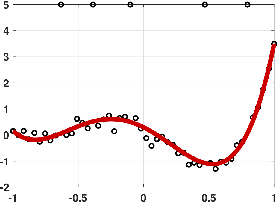
plt.show()The result of this experiment is shown in Figure 7.8. It is remarkable to see that the robust regression result is almost as good as the result would be without outliers.
If robust linear regression performs so well, why don't we use it all the time? Why is least squares regression still more popular? The answer has a lot to do with the computational complexity and the uniqueness of the solution. Linear programming requires an algorithm for a solution. While we have very fast linear programming solvers today, the computational cost of solving a linear program is still much higher than solving a least-squares problem (which is essentially a matrix inversion).
The other issue with robust linear regression is the uniqueness of the solution. Linear programming is known to have degenerate solutions when the constraint set (a high-dimensional polygon) touches the objective function (which is a line) at one of its edges. The least-squares fitting does not have this problem because the optimization surface is a parabola. Unless the matrix \(\mX^T\mX\) is noninvertible, the solution is guaranteed to be the unique global minimum. Linear programming does not have this convenient property. We can have multiple solutions \(\vtheta\) that give the same objective value. If you try to interpret your result by inspecting the magnitude of the \(\vtheta\)'s, the nonuniqueness of the solution would cause problems if linear programming gives you different solutions depending on how the algorithm performs / is initialized.
End of this subsection. Please join us again.
Closing remark. The principle of linear regression is primarily to set up a function to fit the data. This, in turn, is about finding a set of good basis functions and minimizing the appropriate training loss. Selecting the basis is usually done in several ways:
- sep0ex
- The problem forces you to choose certain basis functions. For example, suppose you are working on a disease dataset. The variates are height, weight, and BMI. You do not have any choice here because your goal is to see which factor contributes the most to the cause of the disease.
- There are known basis functions that work. For example, suppose you are working on a speech dataset. Physics tells us that Fourier bases are excellent representations of these sinusoidal functions. So it would make more sense to use the Fourier basis than the polynomials.
- Sometimes the basis can be learned from the data. For example, you can run principal-component analysis (PCA) to extract the basis. Then you can run the linear regression to compute the coefficients. This is a data-driven approach and could apply to some problems.