eBook › Chapter 1 · Mathematical Background

Section 1.2

Approximation

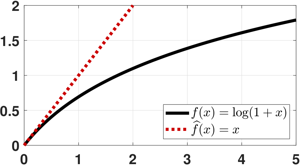
Consider a function $f(x) = \log(1+x)$, for $x > 0$ as shown in Figure 1.5. This is a nonlinear function, and we all know that nonlinear functions are not fun to deal with. For example, if you want to integrate the function $\int_a^b x \log(1+x) \; dx$, then the logarithm will force you to do integration by parts. However, in many practical problems, you may not need the full range of $x > 0$. Suppose that you are only interested in values $x \ll 1$. Then the logarithm can be approximated, and thus the integral can also be approximated.

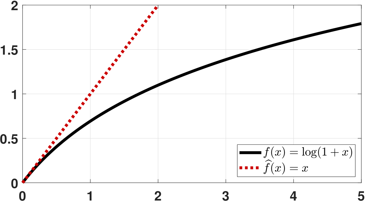
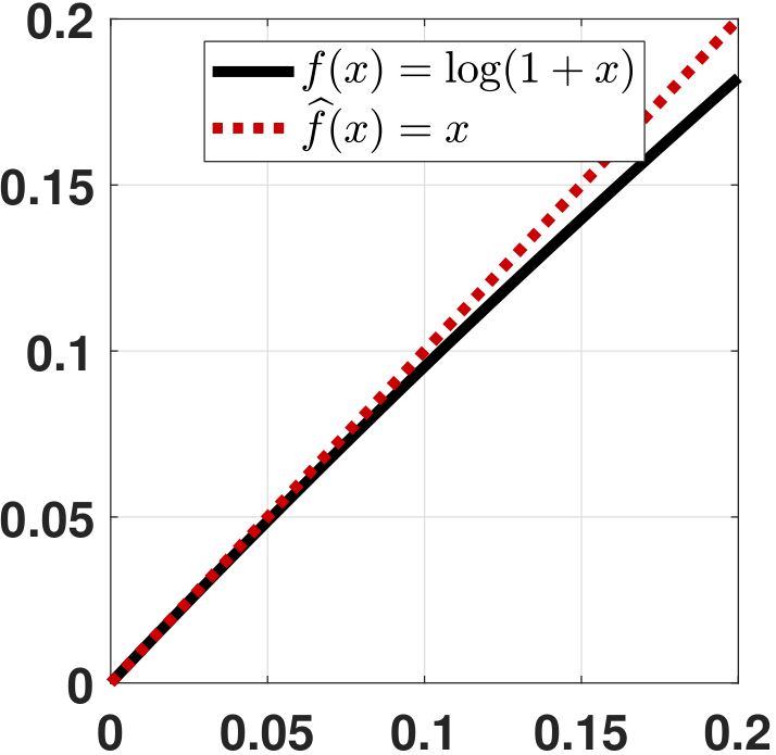
To see how this is even possible, we show in Figure 1.5 the nonlinear function $f(x) = \log(1+x)$ and an approximation $\widehat{f}(x) = x$. The approximation is carefully chosen such that for $x \ll 1$, the approximation $\widehat{f}(x)$ is close to the true function $f(x)$. Therefore, we can argue that for $x \ll 1$,

\log(1+x) \approx x,

thereby simplifying the calculation. For example, if you want to integrate $x\log (1+x)$ for $0 < x < 0.1$, then the integral can be approximated by $\int_0^{0.1} x\log (1+x) \; dx \approx \int_0^{0.1} x^2 \; dx = \frac{x^3}{3} = 3.33 \times 10^{-4}$. (The actual integral is $3.21 \times 10^{-4}$.) In this section, we will learn about the basic approximation techniques. We will use them when we discuss limit theorems in Chapter 6, as well as various distributions, such as from binomial to Poisson.

1.2.1Taylor approximation

Given a function $f: \R \rightarrow \R$, it is often useful to analyze its behavior by approximating $f$ using its local information. Taylor approximation (or Taylor series) is one of the tools for such a task. We will use the Taylor approximation on many occasions.

Definition 1.2 (Taylor Approximation)

Let $f: \R \rightarrow \R$ be a continuous function with infinite derivatives. Let $a \in \R$ be a fixed constant. The Taylor approximation of $f$ at $x = a$ is

\begin{aligned} f(x) &= f(a) + f'(a)(x-a) + \frac{f''(a)}{2!}(x-a)^2 + \cdots \\ &= \sum_{n=0}^{\infty} \frac{f^{(n)}(a)}{n!}(x-a)^n, \end{aligned}

where $f^{(n)}$ denotes the $n$th-order derivative of $f$.

Taylor approximation is a geometry-based approximation. It approximates the function according to the offset, slope, curvature, and so on. According to Definition def:Taylor, the Taylor series has an infinite number of terms. If we use a finite number of terms, we obtain the $n$th-order Taylor approximation:

\begin{aligned} \mbox{First-Order}: \qquad & f(x) = \underset{\textcolor{black}{\text{offset}}}{\underbrace{f(a)}} + \underset{\textcolor{black}{\text{slope}}}{\underbrace{f'(a)(x-a)}} + \calO((x-a)^2)\\ \mbox{Second-Order}: \qquad & f(x) = \underset{\textcolor{black}{\text{offset}}}{\underbrace{f(a)}} + \underset{\textcolor{black}{\text{slope}}}{\underbrace{f'(a)(x-a)}} + \underset{\textcolor{black}{\text{curvature}}}{\underbrace{\frac{f''(a)}{2!}(x-a)^2}} + \calO((x-a)^3). \end{aligned}

Here, the big-O notation $\calO(\varepsilon^k)$ means any term that has an order at least power $k$. For small $\varepsilon$, i.e., $\varepsilon \ll 1$, a high-order term $\calO(\varepsilon^k) \approx 0$ for large $k$.

Example 1.1

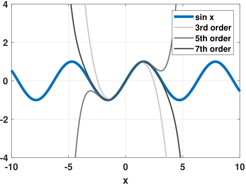
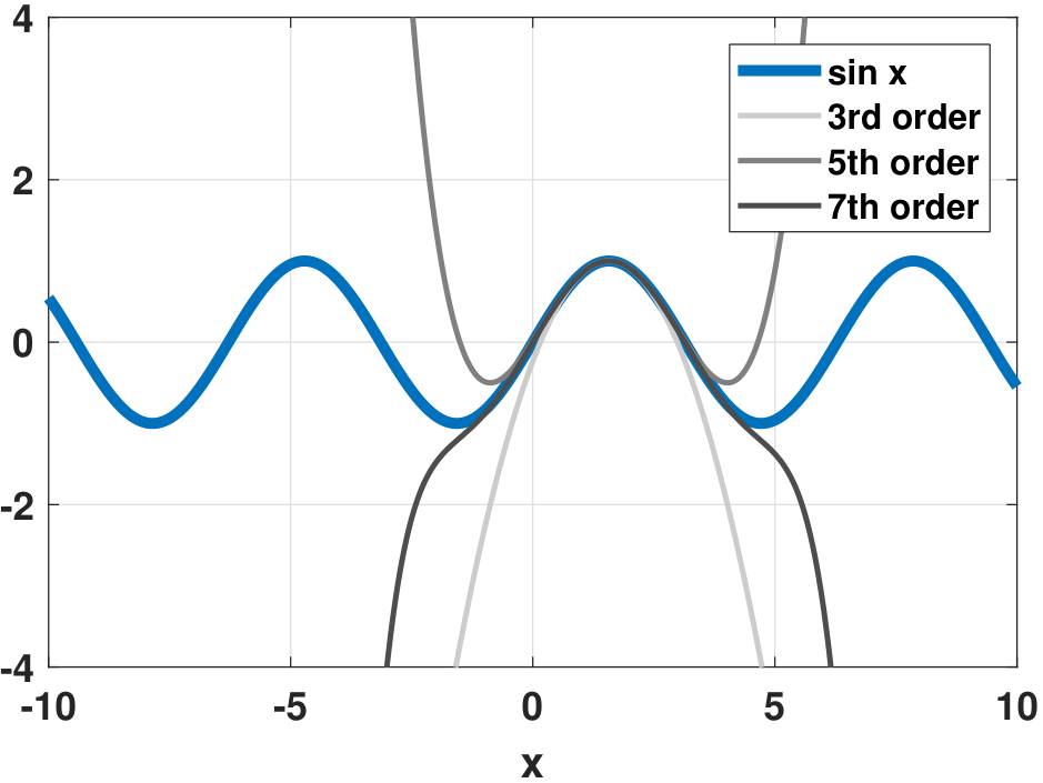
Let $f(x) = \sin x$. Then the Taylor approximation at $x = 0$ is

\begin{aligned} f(x) &\approx f(0) + f'(0)(x-0) + \frac{f''(0)}{2!}(x-0)^2 + \frac{f'''(0)}{3!}(x-0)^3\\ &= \sin(0) + (\cos 0)(x-0) - \frac{\sin(0)}{2!}(x-0)^2 - \frac{\cos(0)}{3!}(x-0)^3 \\ &= 0 + x - 0 - \frac{x^3}{6} = x - \frac{x^3}{6}. \end{aligned}

We can expand further to higher orders, which yields

\begin{aligned} f(x) = x - \frac{x^3}{3!} + \frac{x^5}{5!} - \frac{x^7}{7!} + \cdots \end{aligned}

We show the first few approximations in Figure 1.6.

One should be reminded that Taylor approximation approximates a function $f(x)$ at a particular point $x = a$. Therefore, the approximation of $f$ near $x = 0$ and the approximation of $f$ near $x = \pi/2$ are different. For example, the Taylor approximation at $x = \pi/2$ for $f(x) = \sin x$ is

\begin{aligned} f(x) &= \sin\frac{\pi}{2} + \cos \frac{\pi}{2}\left(x-\frac{\pi}{2}\right) - \frac{\sin\frac{\pi}{2}}{2!}\left(x-\frac{\pi}{2}\right)^2 - \frac{\cos\frac{\pi}{2}}{3!}\left(x-\frac{\pi}{2}\right)^3 \\ &= 1 + 0 - \frac{1}{2}\left(x-\frac{\pi}{2}\right)^2 - 0 = 1 - \frac{1}{2}\left(x-\frac{\pi}{2}\right)^2. \end{aligned}

**Figure 1.6.** Taylor approximation of $f(x) = \sin x$.

1.2.2Exponential series

An immediate application of the Taylor approximation is to derive the exponential series.

Theorem 1.4

Let $x$ be any real number. Then,

e^x = 1 + x + \frac{x^2}{2} + \frac{x^3}{3!} + \cdots = \sum_{k=0}^{\infty} \frac{x^k}{k!}.

Proof. Let $f(x) = e^x$ for any $x$. Then, the Taylor approximation around $x = 0$ is

\begin{aligned} f(x) &= f(0) + f'(0)(x-0) + \frac{f''(0)}{2!}(x-0)^2 + \cdots \\ &= e^0 + e^0(x-0) + \frac{e^0}{2!}(x-0)^2 + \cdots \\ &= 1 + x + \frac{x^2}{2} + \cdots = \sum_{k=0}^\infty \frac{x^k}{k!}. \end{aligned}

■

Practice Exercise 1.5

Evaluate $\displaystyle \sum_{k=0}^{\infty} \frac{\lambda^k e^{-\lambda}}{k!}$.

Solution

\sum_{k=0}^{\infty} \frac{\lambda^k e^{-\lambda}}{k!} = e^{-\lambda} \sum_{k=0}^{\infty} \frac{\lambda^k}{k!} = e^{-\lambda} e^{\lambda} = 1.

This result will be useful for Poisson random variables in Chapter 3.

If we substitute $x = j\theta$ where $j = \sqrt{-1}$, then we can show that

\begin{aligned} \underset{=\cos \theta + j\sin\theta}{\underbrace{e^{j\theta}}} &= 1 + j\theta + \frac{(j\theta)^2}{2!} + \cdots \\ &= \underset{\text{real}}{\underbrace{\left(1 - \frac{\theta^2}{2!} + \frac{\theta^4}{4!} + \cdots\right)}} + j \underset{\text{imaginary}}{\underbrace{\left(\theta - \frac{\theta^3}{3!} + \cdots \right)}} \end{aligned}

Matching the real and imaginary terms, we can show that

\begin{aligned} \cos\theta &= 1 - \frac{\theta^2}{2!} + \frac{\theta^4}{4!} + \cdots\\ \sin\theta &= \theta - \frac{\theta^3}{3!} + \frac{\theta^5}{5!} + \cdots \end{aligned}

This gives the infinite series representations of the two trigonometric functions.

1.2.3Logarithmic approximation

Taylor approximation also allows us to find approximations to logarithmic functions. We start by presenting a lemma.

Lemma 1.1

Let $0 < x < 1$ be a constant. Then,

\log(1+x) = x - \frac{x^2}{2} + \calO(x^3).

Proof. Let $f(x) = \log(1+x)$. Then, the derivatives of $f$ are

f'(x) = \frac{1}{(1+x)}, \quad\mbox{and}\quad f''(x) = -\frac{1}{(1+x)^2}.

Taylor approximation at $x = 0$ gives

\begin{aligned} f(x) &= f(0) + f'(0)(x-0) + \frac{f''(0)}{2}(x-0)^2 + \calO(x^3)\\ &= \log 1 + \left(\frac{1}{(1+0)}\right) x - \left(\frac{1}{(1+0)^2}\right)\frac{x^2}{2} + \calO(x^3)\\ &= x - \frac{x^2}{2} + \calO(x^3). \end{aligned}

■

The difference between this result and the result we showed in the beginning of this section is the order of polynomials we used to approximate the logarithm:

sep0ex
First-order: $\log(1+x) = x$
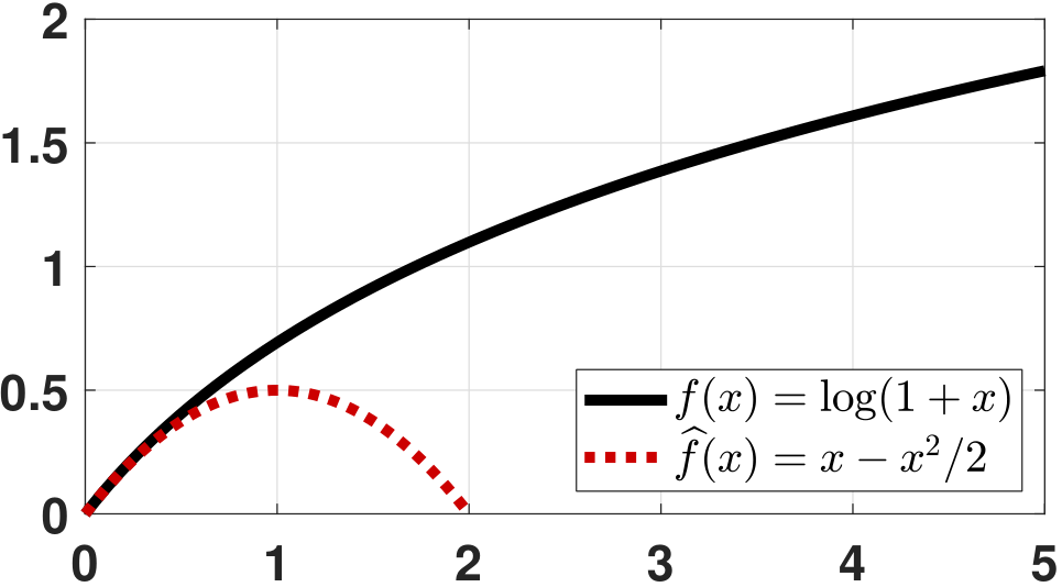
Second-order: $\log(1+x) = x - x^2/2$.

What order of approximation is good? It depends on where you want the approximation to be good, and how far you want the approximation to go. The difference between first-order and second-order approximations is shown in Figure 1.7.

**Figure 1.7.** The function $f(x) = \log(1+x)$, the first-order approximation $\widehat{f}(x) = x$, and the second-order approximation $\widehat{f}(x) = x-x^2/2$.

Example 1.2

When we prove the Central Limit Theorem in Chapter 6, we need to use the following result.

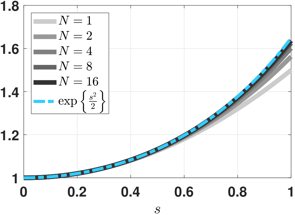
\lim_{N \rightarrow \infty} \left(1+\frac{s^2}{2N}\right)^N = e^{s^2/2}.

The proof of this equation can be done using the Taylor approximation. Consider $N \log\left(1+\frac{s^2}{2N}\right)$. By the logarithmic lemma, we can obtain the second-order approximation:

\log\left(1+\frac{s^2}{2N}\right) = \frac{s^2}{2N} - \frac{s^4}{8N^2}.

Therefore, multiplying both sides by $N$ yields

N \log\left(1+\frac{s^2}{2N}\right) = \frac{s^2}{2} - \frac{s^4}{8N}.

Putting the limit $N \rightarrow \infty$, we can show that

\lim_{N \rightarrow \infty} \left\{ N \log\left(1+\frac{s^2}{2N}\right) \right\} = \frac{s^2}{2}.

Taking the exponential of both sides yields $$\exp\left\{ \lim_{N \rightarrow \infty} N \log \bigg(1+\frac{s^2}{2N}\bigg)\right\} = \exp\left\{\frac{s^2}{2}\right\}.$$ Moving the limit outside the exponential yields the result. Figure 1.8 provides a pictorial illustration.

**Figure 1.8.** We plot a sequence of functions $f_N(x) = \left(1+\frac{s^2}{2N}\right)^N$ and its limit $f(x) = e^{s^2/2}$.