Confidence Interval
The first topic we discuss in this chapter is the confidence interval. At a high level, the confidence interval tells us the quality of our estimator with respect to the number of samples. We begin this section by reviewing the randomness of an estimator. Then we develop the concept of the confidence interval. We discuss several methods for constructing and interpreting these confidence intervals.
9.1.1The randomness of an estimator
Imagine that we have a dataset \(\calX = \{X_1,\ldots,X_N\}\), where we assume that \(X_n\) are i.i.d. copies drawn from a distribution \(f_{X}(x; \theta)\). We want to construct an estimator \(\Thetahat\) of \(\theta\) from the dataset \(\calX\). For example, if \(f_X\) is a Gaussian distribution with an unknown mean \(\theta\), we would like to estimate \(\theta\) using the sample average \(\Thetahat\). In statistics, an estimator \(\Thetahat\) is also known as a statistic, which is constructed from the samples. In this book we use the terms “estimator” and “statistic” interchangeably. Written as equations, an estimator is a function of the samples:
where \(g\) is a function that takes the samples \(X_1,\ldots,X_N\) and returns a random variable \(\Thetahat\). For example, the sample average
is an estimator because it is computed by summing the samples \(X_1,\ldots,X_N\) and dividing it by \(N\).
- sep0ex
An estimator \(\Thetahat\) is a function of the samples \(X_1,\ldots,X_N\):
$$\Thetahat = g(X_1,\ldots,X_N).$$- \(\Thetahat\) is a random variable. It has a PDF, CDF, mean, variance, etc.
By construction, \(\Thetahat\) is a random variable because it is a function of the random samples. Therefore, \(\Thetahat\) has its own PDF, CDF, mean, variance, etc. Since \(\widehat{\Theta}\) is a random variable, we should report both the estimator's value and the estimator's confidence when reporting its performance. The confidence measures the quality of \(\widehat{\Theta}\) when compared to the true parameter \(\theta\). It provides a measure of the reliability of the estimator \(\widehat{\Theta}\). If \(\widehat{\Theta}\) fluctuates a great deal we may not be confident of our estimates. Let's consider the following example.
A class of 1000 students took a test. The distribution of the score is roughly a Gaussian with mean 50 and standard deviation 20. A teaching assistant was too lazy to calculate the true population mean. Instead, he sampled a subset of 5 scores listed as follows:
| Student ID | 1 | 2 | 3 | 4 | 5 |
| Scores | 11 | 97 | 1 | 78 | 82 |
He calculated the average, which is 53.8. This is a very good estimate of the class average (which is 50). What is wrong with his procedure?
He was just lucky. It is quite possible that if he sampled another 5 scores, he would get something very different. For example, if he looks at the 11 to 15 student scores, he could get:
| Student ID | 11 | 12 | 13 | 14 | 15 |
| Scores | 44 | 29 | 19 | 27 | 15 |
In this case the average is 26.8.
Both 53.8 and 26.8 are legitimate estimates, but they are the random realizations of a random variable \(\Thetahat\). This \(\Thetahat\) has a PDF, CDF, mean, variance, etc. It may be misleading to simply report the estimated value from a particular instant, so the confidence of the estimator must be specified.
Distributions of \(\Thetahat\). We next discuss the distribution of \(\Thetahat\). Figure 9.1 illustrates several key ideas. Suppose that the population distribution \(f_X(x)\) is a mixture of two Gaussians. Let \(\theta\) be the mean of this distribution (somewhere between the two peak locations). We sample \(N = 50\) data points \(X_1,\ldots,X_N\) from this distribution. However, the 50 data points we sample today could differ from the 50 data points we sample tomorrow. If we compute the sample average from each of these finite-sample distributions, we will obtain a set of sample averages \(\Thetahat\). Notably, we have a set of \(\Thetahat\) because today we have one \(\Thetahat\) and tomorrow we have another \(\Thetahat\). By plotting the histogram of the sample averages \(\Thetahat\), we will have a distribution.
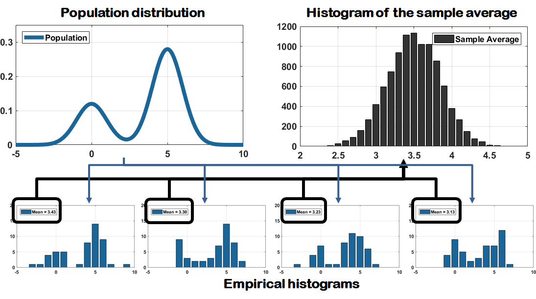
The histogram of \(\Thetahat\) depends on several factors. According to the Central Limit Theorem, the shape of \(f_{\Thetahat}(\theta)\) is a Gaussian because \(\Thetahat\) is the average of \(N\) i.i.d. random variables. If \(\Thetahat\) is not the average of i.i.d. random variables, the shape is not necessarily a Gaussian. This results in additional complications, so we will discuss some tools for dealing with this problem. The spread of the sample distribution is mainly driven by the number of samples we have in each subdataset. As you can imagine, the more samples we have in a subdataset, the more accurate the distribution. Thus you will have a more accurate sample average. The fluctuation of the sample average will also be smaller.
Before we continue, let's summarize the randomness of \(\Thetahat\):
- sep0ex
- \(\Thetahat\) is generated from a finite-sample dataset. Each time we draw a finite-sample dataset, we introduce randomness.
- If \(\Thetahat\) is the sample average, the PDF is (roughly) a Gaussian. If \(\Thetahat\) is not a sample average, the PDF is not necessarily a Gaussian.
- The spread of the fluctuation depends on the number of samples in each sub-dataset.
9.1.2Understanding confidence intervals
The confidence interval is a probabilistic statement about \(\Thetahat\). Instead of studying \(\Thetahat\) as a point, we construct an interval
for some \(\epsilon\) to be determined. Note that this interval is a random interval: If we have a different realization of \(\Thetahat\), we will have a different \(\calI\). We call \(\calI\) the confidence interval for the estimator \(\Thetahat\).
Given this random interval, we ask: What is the probability that \(\calI\) includes \(\theta\)? That means that we want to evaluate the probability
We emphasize that the randomness in this probability is caused by \(\Thetahat\), not \(\theta\). This is because the interval \(\calI\) changes when we conduct a different experiment to obtain a different \(\Thetahat\). The situation is similar to that illustrated on the left-hand side of Figure 9.2. The confidence interval \(\calI\) changes but the true parameter \(\theta\) is fixed.
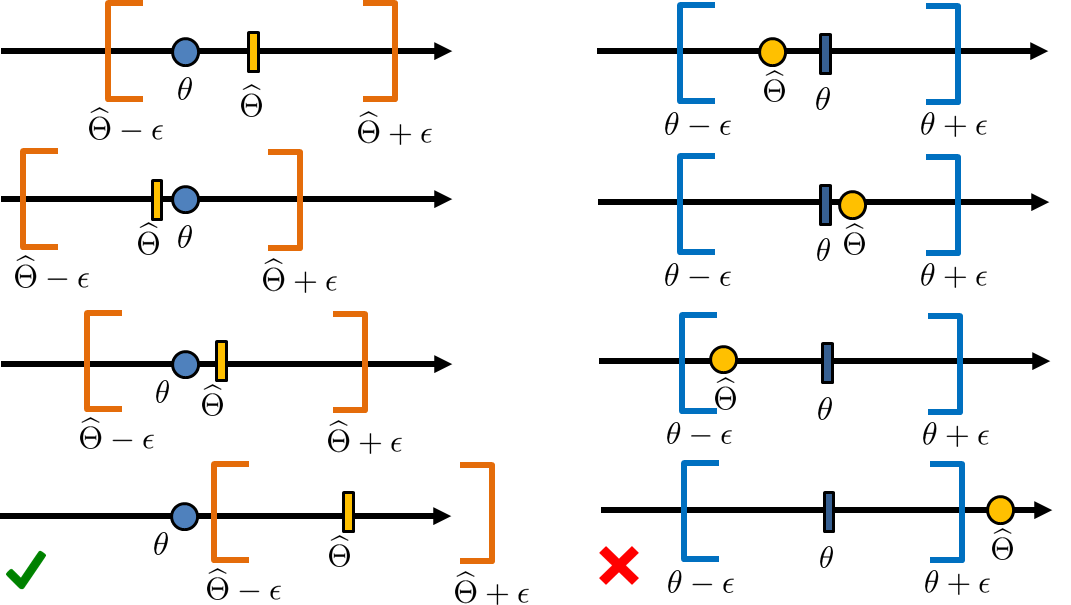
Confidence intervals can be confusing. Often the confusion arises because of the following identity:
Although the values of the two probabilities are the same, the two events are interpreted differently. The right-hand side of Figure 9.2 illustrates \(\Pb[\theta - \epsilon \le \Thetahat \le \theta + \epsilon]\). The interval \([\theta-\epsilon,\theta+\epsilon]\) is fixed. What is the probability that the estimator \(\Thetahat\) lies within this deterministic interval? To find this probability, we need to know the true parameter \(\theta\), which is not available. By contrast, the other probability \(\Pb[\Thetahat-\epsilon \le \theta \le \Thetahat+\epsilon]\) does not require any knowledge about the true parameter \(\theta\). What is the probability that the true parameter is included inside the random interval? If the probability is high, we say that there is a good chance that our confidence interval will contain the true parameter. This is observed in the left-hand side of Figure 9.2.
In practice we often set \(\Pb[\Thetahat-\epsilon \le \theta \le \Thetahat+\epsilon]\) to be greater than a certain confidence level, say 95%, and then we determine \(\epsilon\). Once we have determined \(\epsilon\), we can claim that with 95% probability the interval \([\Thetahat - \epsilon, \; \Thetahat + \epsilon]\) will include the unknown parameter \(\theta\). We do not need to know \(\theta\) at any point in this process.
To make this more general, we define \(1-\alpha\) as the confidence level for some parameter \(\alpha\). For example, if we would like to have a 95% confidence level, we set \(\alpha = 0.05\). Then the probability inequality
tells us that there is at least a 95% chance that the random interval \(\calI = [\Thetahat - \epsilon, \;\; \Thetahat + \epsilon]\) will include the true parameter \(\theta\). In this case we say that \(\calI\) is a “95% confidence interval”.
- sep0ex
- It is a random interval \([\Thetahat-\epsilon, \Thetahat+\epsilon]\) such that there is a 95% probability for it to include the true parameter \(\theta\).
- It is not the deterministic interval \([\theta-\epsilon,\theta+\epsilon]\), because we never know \(\theta\).
After analyzing the life expectancy of people in the United States, it was concluded that the 95% confidence interval is (77.8, 79.1) years old. Is the following claim valid?
About 95% of the people in the United States have a life expectancy between 77.8 years old and 79.1 years old.
No. The confidence interval tells us that with 95% probability the random interval \((77.8, 79.1)\) will include the true average. We emphasize that \((77.8, 79.1)\) is random because it is constructed from a small set of data points. If we survey another set of people we will have another interval.
Since we do not know the true average, we do not know the percentage of people whose life expectancy is between 77.8 years old and 79.1 years old. It could be that the true average is 80 years old, which is out of the range. It could also be that the true average is 77.9 years old, which is within the range, but only \(10\%\) of the population may have life expectancy in \((77.8, 79.1)\).
After studying the SAT scores of 1000 high school students, it was concluded that the 95% confidence interval is (1134, 1250) points. Is the following claim valid?
There is a 95% probability that the average SAT score in the population is in the range 1134 and 1250.
Yes, but it can be made clearer. The average SAT score in the population remains unknown. It is a constant and it is deterministic, so there is no probability associated with it. A better way to say this is: “There is a 95% probability that the random interval 1134 and 1250 will include the average SAT score.” We emphasize that the 95% probability is about the random interval, not the unknown parameter.
9.1.3Constructing a confidence interval
Let's consider an example. Suppose that we have a set of i.i.d. observations \(X_1,\ldots,X_N\) that are Gaussians with an unknown mean \(\theta\) and a known variance \(\sigma^2\). We consider the maximum-likelihood estimator, which is the sample average:
Our goal is to construct a confidence interval.
Before we consider the equations, let's look at a graph illustrating what we want to achieve. Figure 9.3 shows a population distribution, which is a Gaussian in this example.
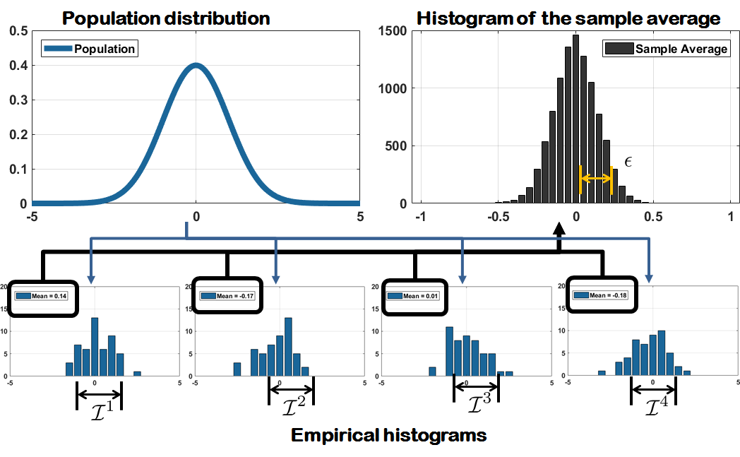
We draw \(N\) samples from the Gaussian to construct a random subset. Based on this random subset we construct the estimator \(\Thetahat\). Since this estimator is based on the particular random subset we have, we can follow the same approach by drawing another random subset. To differentiate the estimators constructed by the different random subsets, let's call the estimators \(\Thetahat^{(1)}\) and \(\Thetahat^{(2)}\), respectively. For each estimator we construct an interval \([\Thetahat-\epsilon, \; \Thetahat+\epsilon]\) to obtain two different intervals:
If we can determine \(\epsilon\), we have found the confidence interval.
We can determine the confidence interval by observing the histogram of \(\Thetahat\), which in our case is the histogram of the sample average, since the histogram of \(\Thetahat\) is well-defined, especially if we are looking at the sample average. The histogram of the sample average is a Gaussian because the average of \(N\) i.i.d. Gaussian random variables is Gaussian. Therefore, the width of this Gaussian is determined by the answer to this question:
For what \(\epsilon\) can we cover 95% of the histogram of \(\Thetahat\)?
To find the answer, we set up the following probability inequality:
This probability says that we want to find an \(\epsilon\) such that the majority of \(\Thetahat\) is living close to its mean. The level \(1-\alpha\) is our confidence level, which is typically 95%. Equivalently, we let \(\alpha = 0.05\).
In the above equation, we can define the quotient as
We know that \(\widehat{Z}\) is a zero-mean unit-variance Gaussian because it is the standardized variable. [Note: Not all normalized variables are Gaussian, but if \(\Thetahat\) is a Gaussian the normalized variable will remain a Gaussian.] Thus, the probability inequality we are looking at is
The PDF of \(\widehat{Z}\) is shown in Figure 9.4. As you can see, to achieve 95% confidence we need to pick an appropriate \(\epsilon\) such that the shaded area is less than 5%.
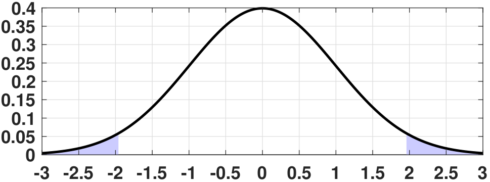
Since \(\Pb[\widehat{Z} \le \epsilon]\) is the CDF of a Gaussian, it follows that
Using the symmetry of the Gaussian, it follows that \(\Phi\left(-\epsilon\right) = 1-\Phi\left(\epsilon \right)\) and hence
Equating this result with the probability inequality \(\Pb[|\widehat{Z}| \le \epsilon] \ge 1-\alpha\), we have that
The remainder of this problem is solvable on a computer. On MATLAB, we can call icdf to compute the inverse CDF of a standard Gaussian. On Python, the command is stats.norm.ppf. The commands are as shown below.
% MATLAB code to compute the width of the confidence interval
    alpha = 0.05;
    mu = 0; sigma = 1; % Standard Gaussian
epsilon = icdf('norm',1-alpha/2,mu,sigma)# Python code to compute the width of the confidence interval
import scipy.stats as stats
alph = 0.05;
mu = 0; sigma = 1; # Standard Gaussian
epsilon = stats.norm.ppf(1-alph/2, mu, sigma)
print(epsilon)If everything is done properly, we see that for a 95% confidence level (\(\alpha = 0.05\)) the corresponding \(\epsilon\) is \(\epsilon = 1.96\).
After determining \(\epsilon\), it remains to determine \(\E[\Thetahat]\) and \(\Var[\Thetahat]\) in order to complete the probability inequality. To this end, we note that
if we assume that the population distribution is \(\text{Gaussian}(\theta,\sigma^2)\), where \(\theta\) is unknown but \(\sigma\) is known. Substituting these into the probability inequality, we have that
where we let \(\epsilon = 1.96\) for a 95% confidence level. Therefore, the 95% confidence interval is
As you can see, we do not need to know the value of \(\theta\) at any point of the derivation because the confidence interval in Eq. (9.5) does not involve \(\theta\). This is an important difference with the other probability \(\Pb[\theta-\epsilon \le \Thetahat \le \theta+\epsilon]\), which requires \(\theta\).
- sep0ex
- Compute the estimator \(\widehat{\Theta}\).
- Determine the width of the confidence interval \(\epsilon\) by inspecting the confidence level \(1-\alpha\). If \(\widehat{\Theta}\) is Gaussian, then \(\epsilon = \Phi^{-1}(1-\frac{\alpha}{2})\).
- If \(\Thetahat\) is not a Gaussian, replace the Gaussian CDF by the CDF of \(\Thetahat\).
- The confidence interval is \([\Thetahat -\epsilon, \; \Thetahat + \epsilon]\).
9.1.4Properties of the confidence interval
Some important properties of the confidence interval are listed below.
- sep0ex
Probability of \(\Thetahat\) is the same as probability of \(\widehat{Z}\). First, the two random variables \(\Thetahat\) and \(\widehat{Z}\) have a one-to-one correspondence. We proved the following in Chapter 6:
If \(\Thetahat \sim \text{Gaussian}(\theta,\frac{\sigma^2}{N})\), then
$$\widehat{Z} \bydef \frac{\Thetahat-\theta}{\sigma/\sqrt{N}} \sim \text{Gaussian}(0,1).$$For example, if \(\Thetahat \sim \text{Gaussian}(\theta,\frac{\sigma^2}{N})\) with \(N = 1\), \(\theta = 1\) and \(\sigma = 2\), then a 95% confidence level is
$$\begin{aligned} 0.95 &\approx \Pb[-1.96 \le \widehat{Z} \le 1.96],\qquad \text{\textcolor{black}{($\widehat{Z}$ is within 1.96 std from $\widehat{Z}$'s mean)}}\\ &= \Pb[-1.96 \le \frac{\Thetahat-\theta}{\sigma/\sqrt{N}} \le 1.96]\\ &= \Pb\left[\theta-1.96\frac{\sigma}{\sqrt{N}} \le \Thetahat \le \theta+1.96\frac{\sigma}{\sqrt{N}}\right]\\ &= \Pb[-2.92 \le \Thetahat \le 4.92]. \qquad \text{\textcolor{black}{($\Thetahat$ is within 1.96 std from $\Thetahat$'s mean)}} \end{aligned}$$Note that while the range for \(\widehat{Z}\) is different from the range for \(\Thetahat\), they both return the same probability. The only difference is that \(\Thetahat\) is constructed before the normalization and \(\widehat{Z}\) is constructed after the normalization.
Standard error. In this estimation problem we know that \(\Thetahat\) is the sample average. We assume that the mean \(\theta\) is unknown but the variance \(\Var[\Thetahat]\) is known. The standard deviation of \(\Thetahat\) is called the standard error:
$$\text{\textsf{se}} = \sqrt{\Var[\Thetahat]} = \frac{\sigma}{\sqrt{N}}.$$Critical value. The value \(1.96\) in our example is often known as the critical value. It is defined as
$$z_\alpha = \Phi^{-1}\left(1-\frac{\alpha}{2}\right).$$The \(z_\alpha\) value gives us a multiplier applied to the standard error that will result in a value within the confidence interval. This is because, by the definition of the confidence interval, the interval is
$$\begin{aligned} \left[\Thetahat - 1.96 \frac{\sigma}{\sqrt{N}}, \quad \Thetahat + 1.96 \frac{\sigma}{\sqrt{N}}\right] = \left[\Thetahat - z_\alpha\text{\textsf{se}}, \quad \Thetahat + z_\alpha\text{\textsf{se}} \right] \end{aligned}$$
- sep0ex
Margin of error. The margin of error is defined as
$$\text{margin of error} = z_\alpha \frac{\sigma}{\sqrt{N}}.$$The margin of error is also the width of the confidence interval. As the name implies, the margin of error tells us how much error the confidence interval includes when predicting the population parameter.
Suppose that the number of photos a Facebook user uploads per day is a random variable with \(\sigma = 2\). In a set of 341 users, the sample average is 2.9. Find the 90% confidence interval of the population mean.
We set \(\alpha = 0.1\). The \(z_\alpha\)-value is
The 90% confidence interval is then
Therefore, with 90% probability, the interval \([2.72, 3.08]\) includes the population mean.
Professional cyber-athletes have a standard deviation of \(\sigma = 73.4\) actions per minute. If we want to estimate the average actions per minute of the population, how many samples are needed to obtain a margin of error \(<20\) at 90% confidence?
With a 90% confidence level, the \(z_\alpha\)-value is
The margin of error is 20. So we have \(z_\alpha \frac{\sigma}{\sqrt{N}} = 20\). Moving around the terms gives us
Therefore, we need at least \(N = 37\) samples to ensure a margin of error of \(< 20\) at a 90% confidence level.
The concepts of standard error se, the \(z_\alpha\) value, and the margin of error are summarized in Figure 9.5.
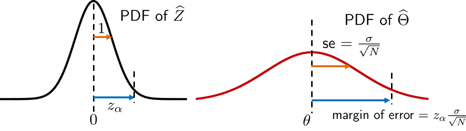
The left-hand side is the PDF of \(\widehat{Z}\). It is the normalized random variable, which is also the standard Gaussian. The right-hand side is the PDF of \(\Thetahat\), the unnormalized random variable. The \(z_\alpha\) value is located in the \(\widehat{Z}\)-space. It defines the range of \(\widehat{Z}\) in the PDF within which we are confident about the true parameter. The corresponding value in the \(\Thetahat\)-space is the margin of error. This is found by multiplying \(z_\alpha\) with the standard deviation of \(\Thetahat\), known as the standard error. Correspondingly, in the \(\widehat{Z}\)-space the standard deviation is unity.
Two further points about the confidence interval should be mentioned:
- sep0ex
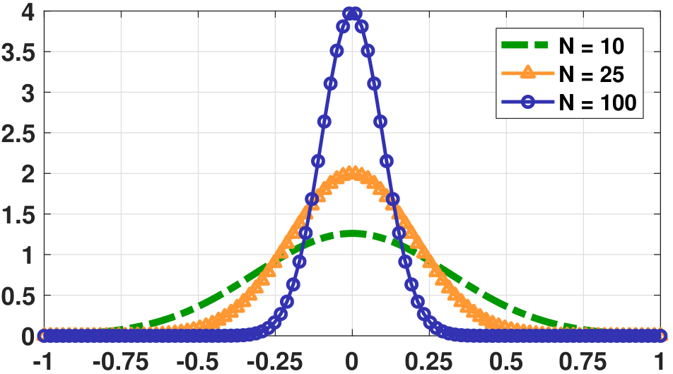
Number of Samples \(N\). The confidence interval is a function of \(N\). As we increase the number of samples, the distribution of the estimator \(\Thetahat\) becomes narrower. Specifically, if \(\Thetahat\) follows a Gaussian distribution
$$\Thetahat \sim \text{Gaussian}\left(\theta, \;\; \frac{\sigma^2}{N}\right),$$then \(\Thetahat \overset{p}{\rightarrow} \theta\) as \(N \rightarrow \infty\). Figure 9.6 illustrates a few examples of \(\Thetahat\) as \(N\) grows. In the limit when \(N \rightarrow \infty\), we observe that the interval becomes
$$\left[\Thetahat - 1.96 \frac{\sigma}{\sqrt{N}}, \quad \Thetahat + 1.96 \frac{\sigma}{\sqrt{N}}\right] \longrightarrow \left[\Thetahat, \quad \Thetahat\right] = \Thetahat.$$In this case, the statement \(\theta \in \left[\Thetahat - 1.96 \frac{\sigma}{\sqrt{N}}, \quad \Thetahat + 1.96 \frac{\sigma}{\sqrt{N}}\right]\) becomes \(\theta = \Thetahat\). That means the estimator \(\Thetahat\) returns the correct true parameter \(\theta\). Of course, it is possible that \(\E[\Thetahat] \not= \theta\), i.e., the estimator is biased. In that case, having more samples will cause the estimator to approach another estimate that is not \(\theta\).
- sep0ex
Distribution of \(\widehat{Z}\). When defining the confidence interval we constructed an intermediate variable
$$\widehat{Z} = \frac{\Thetahat - \theta}{\sigma/\sqrt{N}}.$$Since \(X_n\)'s are i.i.d. Gaussian, it follows that \(\widehat{Z}\) is also Gaussian. This gives us a way to calculate the probability using the standard Gaussian table. What happens when \(X_n\)'s are not Gaussian? The good news is that even if \(X_n\)'s are not Gaussian, for sufficiently large \(N\), the random variable \(\Thetahat\) is more or less Gaussian, because of the Central Limit Theorem. Therefore, even if \(X_n\)'s are not Gaussian we can still use the Gaussian probability table to construct \(\alpha\) and \(\epsilon\).
9.1.5Student's \(t\)-distribution
In the discussions above, we estimate the population mean \(\theta\) using the estimator \(\Thetahat\). The assumption was that the variance \(\sigma^2\) was known a priori and hence is fixed. In practice, however, there are many situations where \(\sigma^2\) is not known. Thus we not only need to use the mean estimator \(\Thetahat\) but also the variance estimator \(\widehat{S}\), which can be defined as
where \(\Thetahat\) is the estimator of the mean. What is the confidence interval for \(\Thetahat\)?
For a confidence interval to be valid, we expect it to take the form of
which is essentially the confidence interval we have just derived but with \(\sigma\) replaced by \(\widehat{S}\). However, there is a problem with this. When we derive the confidence interval assuming a known \(\sigma\), the \(z_\alpha\) value is determined by checking the standard Gaussian
which gives us \(z_\alpha = \Phi^{-1}(1-\alpha/2)\). The whole derivation is based on the fact that \(\widehat{Z}\) is a standard Gaussian. Now that we have replaced \(\sigma\) by \(\widehat{S}\), the new random variable
is not a standard Gaussian.
It turns out that the distribution of \(T\) is Student's \(t\)-distribution with \(N-1\) degrees of freedom. The PDF of Student's \(t\)-distribution is given as follows.
If \(X\) is a random variable following Student's \(t\)-distribution of \(\nu\) degrees of freedom, then the PDF of \(X\) is
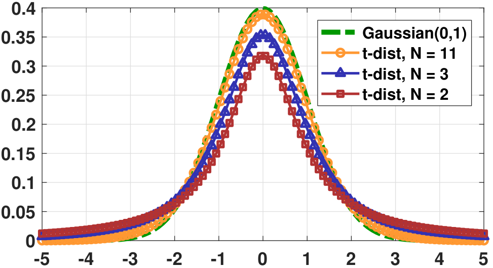
We may compare Student's \(t\)-distribution with the Gaussian distribution. Figure 9.7 shows the standard Gaussian and several \(t\) distributions with \(\nu = N-1\) degrees of freedom. Note that Student's \(t\)-distribution has a similar shape to the Gaussian but it has a heavier tail.
Since \(T = \frac{\Thetahat - \theta}{\widehat{S}/\sqrt{N}}\) is a \(t\)-random variable, to determine the \(z_\alpha\) value we can follow the same procedure by considering the CDF of \(T\). Let the CDF of the Student's \(t\)-distribution with \(\nu\) degrees of freedom be
If we want \(\Pb[|T| \le z_\alpha] = 1-\alpha\), it follows that
Therefore, the new confidence interval, assuming an unknown \(\widehat{S}\), is
with \(z_\alpha\) defined in Eq. (9.12), using \(\nu = N-1\).
A survey asked \(N = 14\) people for their rating of a movie. Assume that the mean estimator is \(\Thetahat\) and the variance estimator is \(\widehat{S}\). Find the confidence interval.
If we use Student's \(t\)-distribution, it follows that
where the degrees of freedom are \(\nu = 14-1 = 13\). Thus the confidence interval is
The MATLAB and Python codes to report the \(z_\alpha\) value of a Student's \(t\)-distribution are shown below. They are both called through the inverse CDF function. In MATLAB it is icdf, and in Python it is stats.t.ppf.
% MATLAB code to compute the z_alpha value of t distribution
    alpha = 0.05;
    nu = 13;
z = icdf(‘t’,1-alpha/2,nu)# Python code to compute the z_alpha value of t distribution
import scipy.stats as stats
alph = 0.05
nu = 13
z = stats.t.ppf(1-alph/2, nu)
print(z)A class of 10 students took a midterm exam. Their scores are given in the following table.
| Student | 1 | 2 | 3 | 4 | 5 | 6 | 7 | 8 | 9 | 10 |
| Score | 72 | 69 | 75 | 58 | 67 | 70 | 60 | 71 | 59 | 65 |
Find the 95% confidence interval.
The mean and standard deviation of the datasets are respectively \(\Thetahat = 66.6\) and \(\widehat{S} = 5.91\). The critical \(z_\alpha\) value is determined by Student's \(t\)-distribution:
The confidence interval is
Therefore, with 95% probability, the interval \(\left[62.37, 70.83\right]\) will include the true population mean.
Remark 1. Make sure you understand the meaning of “population mean” in this example. Since we have ten students, isn't the population mean just the average of the ten scores? This is incorrect. In statistics, we assume that these ten students are the realizations of some underlying (unknown) random variable \(X\) with some PDF \(f_X(x)\). The population mean \(\theta\) is therefore the expectation \(\E[X]\), where the expectation is taken w.r.t. \(f_X\). The sample average \(\Thetahat\), which is the average of the ten numbers, is an estimator of the population mean \(\theta\).
Remark 2. You may be wondering why we are using Student's \(t\)-distribution here when we do not even know the PDF of \(X\). The answer is that it is an approximation. When \(X\) is Gaussian, the sample average \(\Thetahat\) is a Student's \(t\)-distribution, assuming that the variance is approximated by the sample variance \(\widehat{S}\). This result is attributed to the original paper of William Gosset, who developed Student's \(t\)-distribution.
The above example can be solved computationally. An implementation of Python is given below, and the MATLAB implementation is straightforward.
# Python code to generate a confidence interval
    import numpy as np
    import scipy.stats as stats
    x = np.array([72, 69, 75, 58, 67, 70, 60, 71, 59, 65])
    N         = x.size
    Theta_hat = np.mean(x) # Sample mean
    S_hat     = np.std(x)  # Sample standard deviation
    nu        = x.size-1   # degrees of freedom
    alpha     = 0.05       # confidence level
    z    = stats.t.ppf(1-alph/2, nu)
    CI_L = Theta_hat-z*S_hat/np.sqrt(N)
    CI_U = Theta_hat+z*S_hat/np.sqrt(N)
print(CI_L, CI_U)- sep0ex
- It was developed by William Gosset in 1908. When he published the paper he used the pseudonym Student.
- We use Student's \(t\)-distribution to model the estimator \(\Thetahat\)'s PDF when the variance \(\sigma^2\) is replaced by the sample variance \(\widehat{S}^2\).
- Student's \(t\)-distribution has a heavier tail than a Gaussian.
9.1.6Comparing Student's \(t\)-distribution and Gaussian
We now discuss an important theoretical result regarding the relationship between a Student's \(t\)-distribution and Gaussian distribution. The main result is that the standard Gaussian is a limiting distribution of the \(t\) distribution as the degrees of freedom \(\nu \rightarrow \infty\).
As \(\nu \rightarrow \infty\), the Student's \(t\)-distribution approaches the standard Gaussian distribution:
The proof of the theorem requires Stirling's approximation, which is not essential for this book. Feel free to skip it if needed.
Proof. There are two results we need to use:
- sep0ex
- Stirling's approximation: (K. G. Binmore, Mathematical analysis: A straightforward approach. Cambridge University Press, 1977. Section 17.7.2.) \(\Gamma(z) \approx \sqrt{\frac{2\pi}{z}}\left(\frac{z}{e}\right)^z\).
- Exponential approximation: \((1+\frac{x}{k})^{-k} \rightarrow e^{-x}\), as \(k \rightarrow \infty\).
We have that
Putting a limit of \(\nu \rightarrow \infty\), we have that
The other limit follows from the fact that
Combining the two limits proves the theorem.
■End of the proof. Please join us again.
This theorem has several implications:
- sep0ex
- When \(N\) is large, \(S^2 \rightarrow \sigma^2\). The Gaussian approximation kicks in, and so Student's \(t\)-distribution is more or less the same as the Gaussian.
- Student's \(t\)-distribution is better for small \(N\), usually \(N \le 30\). If \(N \ge 30\), using the Gaussian approximation suffices.
- If \(X\) is Gaussian, Student's \(t\)-distribution is an excellent model. If \(X\) is not Gaussian, Student's \(t\)-distribution will have some issues unless \(N\) increases.