eBook › Chapter 4 · Continuous Random Variables

Section 4.1

Probability Density Function

4.1.1Some intuitions about probability density functions

Let's begin by outlining some intuitive reasoning, which is needed to define the probability of continuous events properly. These intuitions are based on the fact that probability is a measure. In the following discussion, you will see a sequence of logical arguments for constructing such a measure for continuous events. Some arguments are discussed in Chapter 2, but now we place them in the context of continuous random variables.

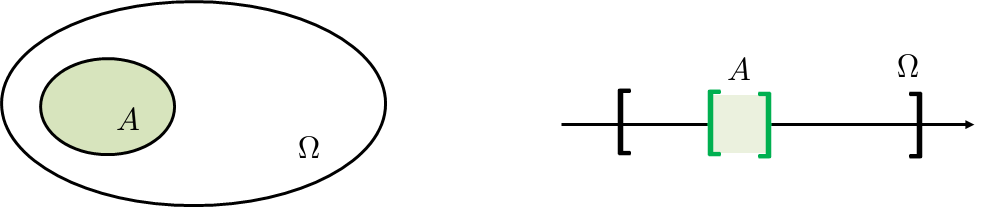
Suppose we are given an event $A$ that is a subset in the sample space $\Omega$, as illustrated in Figure 4.1. In order to calculate the probability of $A$, the measure perspective suggests that we consider the relative size of the set

\begin{aligned} \Pb[ \{x \in A\} ] = \frac{\text{``size'' of }A}{\text{``size'' of }\Omega}. \end{aligned}

The right-hand side of this equation captures everything about the probability: It is a measure of the size of a set. It is relative to the sample space. It is a number between 0 and 1. It can be applied to discrete sets, and it can be applied to continuous sets.

**Figure 4.1.** [Left] An event $A$ in the sample space $\Omega$. The probability that $A$ happens can be calculated as the “size” of $A$ relative to the “size” of $\Omega$. [Right] A specific example on the real line. Note that the same definition of probability applies: The probability is the size of the interval $A$ relative to that of the sample space $\Omega$.

How do we measure the “size” of a continuous set? One possible way is by means of integrating the length, area, or volume covered by the set. Consider an example: Suppose that the sample space is the interval $\Omega = [0,5]$ and the event is $A = [2,3]$. To measure the “size” of $A$, we can integrate $A$ to determine the length. That is,

\Pb[ \{x \in [2,3]\} ] = \frac{\text{``size'' of }A}{\text{``size'' of }\Omega} = \frac{\int_{A} \;dx}{\int_{\Omega} \;dx} = \frac{\int_2^3 \;dx}{\int_0^5 \;dx} = \frac{1}{5}.

Therefore, we have translated the “size” of a set to an integration. However, this definition is a very special case because when we calculate the “size” of a set, we treat all the elements in the set with equal importance. This is a strong assumption that will be relaxed later. But if you agree with this line of reasoning, we can rewrite the probability as

\begin{aligned} \Pb[ \{x \in A\} ] = \frac{\int_{A} \;dx}{\int_{\Omega} \;dx} &= \frac{\int_{A} \;dx}{|\Omega|} \\ &= \int_A \underset{\textcolor{black}{\text{equally important over }\Omega}}{\underbrace{\quad \frac{1}{|\Omega|} \quad}} \;dx. \end{aligned}

This equation says that under our assumption (that all elements are equiprobable), the probability of $A$ is calculated as the integration of $A$ using an integrand $1/|\Omega|$ (note that $1/|\Omega|$ is a constant with respect to $x$). If we evaluate the probability of another event $B$, all we need to do is to replace $A$ with $B$ and compute $\int_B \frac{1}{|\Omega|}\;dx$.

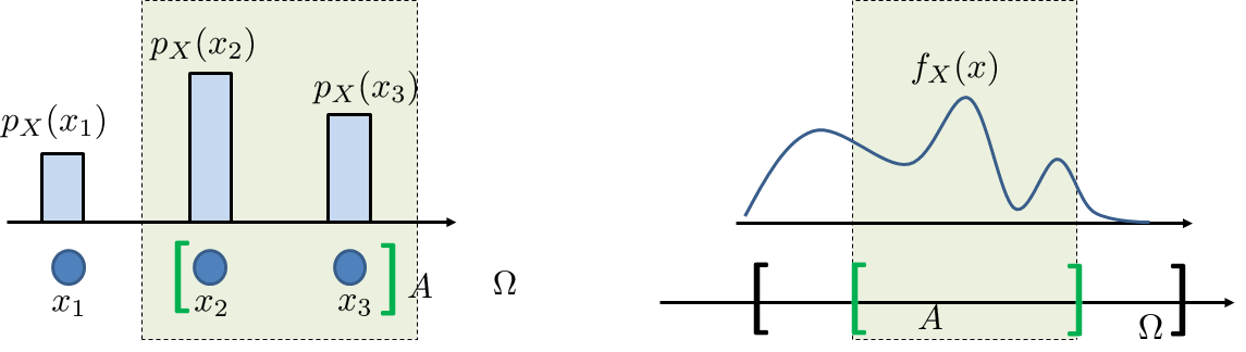
What happens if we want to relax the “equiprobable” assumption? Perhaps we can adopt something similar to the probability mass function (PMF). Recall that a PMF $p_X$ evaluated at a point $x$ is the probability that the state $x$ happens, i.e., $p_X(x) = \Pb[X = x]$. So, $p_X(x)$ is the relative frequency of $x$. Following the same line of thinking, we can define a function $f_X$ such that $f_X(x)$ tells us something related to the “relative frequency”. To this end, we can treat $f_X$ as a continuous histogram with infinitesimal bin width as shown in Figure 4.2. Using this $f_X$, we can replace the constant function $1/|\Omega|$ with the new function $f_X(x)$. This will give us

\Pb[ \{x \in A\} ] = \int_A \underset{\textcolor{black}{\text{replace $1/|\Omega|$ }}}{\underbrace{\quad f_X(x) \quad}} \;dx.

If we compare it with a PMF, we note that when $X$ is discrete,

\Pb[ \{x \in A\} ] = \sum_{x \in A} p_X(x).

Hence, $f_X$ can be considered a continuous version of $p_X$, although we do not recommend this way of thinking for the following reason: $p_X(x)$ is a legitimate probability, but $f_X(x)$ is not a probability. Rather, $f_X$ is the probability per unit length, meaning that we need to integrate $f_X$ (times $dx$) in order to generate a probability value. If we only look at $f_X$ at a point $x$, then this point is a measure-zero set because the length of this set is zero.

Eq. (4.1) should be familiar to you from Chapter 2. The function $f_X(x)$ is precisely the weighting function we described in that chapter.

**Figure 4.2.** [Left] A probability mass function (PMF) tells us the relative frequency of a state when computing the probability. In this example, the “size” of $A$ is $p_X(x_2)+p_X(x_3)$. [Right] A probability density function (PDF) is the infinitesimal version of the PMF. Thus, the “size” of $A$ is the integration over the PDF.

What is a PDF?

sep0ex
A PDF is the continuous version of a PMF.
We integrate a PDF to compute the probability.
We integrate instead of sum because continuous events are not countable.

To summarize, we have learned that when measuring the size of a continuous event, the discrete technique (counting the number of elements) does not work. Generalizing to continuous space requires us to integrate the event. However, since different elements in an event have different relative emphases, we use the probability density function $f_X(x)$ to tell us the relative frequency for a state $x$ to happen. This PDF serves the role of the PMF.

4.1.2More in-depth discussion about PDFs

A continuous random variable $X$ is defined by its probability density function $f_X$. This function has to satisfy several criteria, summarized as follows.

Definition 4.1

A probability density function $f_X$ of a random variable $X$ is a mapping $f_X: \Omega \rightarrow \R$, with the properties

sep0ex
Non-negativity: $f_X(x) \ge 0$ for all $x \in \Omega$
Unity: $\int_{\Omega} f_X(x)\;dx = 1$
Measure of a set: $\Pb[\{x \in A\}] = \int_A f_X(x) \;dx$

If all elements of the sample space are equiprobable, then the PDF is $f(x) = 1/|\Omega|$. You can easily check that it satisfies all three criteria.

Let us take a closer look at the three criteria:

sep0ex
Non-negativity: The non-negativity criterion $f_X(x) \ge 0$ is reminiscent of Probability Axiom I. It says that no matter what $x$ we are looking at, the probability density function $f_X$ evaluated at $x$ should never give a negative value. Axiom I ensures that we will not get a negative probability.
Unity: The unity criterion $\int_{\Omega} f(x) \;dx = 1$ is reminiscent of Probability Axiom II, which says that measuring over the entire sample space will give 1.
Measure of a set: The third criterion gives us a way to measure the size of an event $A$. It says that since each $x \in \Omega$ has a different emphasis when calculating the size of $A$, we need to scale the elements properly. This scaling is done by the PDF $f_X(x)$, which can be regarded as a histogram with a continuous $x$-axis. The third criterion is a consequence of Probability Axiom III, because if there are two events $A$ and $B$ that are disjoint, then $\Pb[\{x \in A\} \cup \{x \in B\}] = \int_A f_X(x) \;dx + \int_B f_X(x) \;dx$ because $f_X(x) \ge 0$ for all $x$.

If the random variable $X$ takes real numbers in 1D, then a more “user-friendly” definition of the PDF can be given.

Definition 4.2

Let $X$ be a continuous random variable. The probability density function (PDF) of $X$ is a function $f_X: \Omega \rightarrow \R$ that, when integrated over an interval $[a,\,b]$, yields the probability of obtaining $a \le X \le b$:

\Pb[a \le X \le b] = \int_{a}^{b} f_X(x) \;dx.

This definition is just a rewriting of the previous definition by explicitly writing out the definition of $A$ as an interval $[a,b]$. Here are a few examples.

Example 4.1

Let $f_X(x) = 3x^2$ with $\Omega = [0,1]$. Let $A = [0,0.5]$. Then the probability $\Pb[\{X \in A\}]$ is

\begin{aligned} \Pb[0 \le X \le 0.5] = \int_{0}^{0.5} 3x^2 \;dx = \frac{1}{8}. \end{aligned}

Example 4.2

Let $f_X(x) = 1/|\Omega|$ with $\Omega = [0,5]$. Let $A = [3,5]$. Then the probability $\Pb[\{X \in A\}]$ is

\begin{aligned} \Pb[3 \le X \le 5] = \int_{3}^{5} \frac{1}{|\Omega|} \;dx = \int_3^5 \frac{1}{5} \;dx = \frac{2}{5}. \end{aligned}

Example 4.3

Let $f_X(x) = 2 x$ with $\Omega = [0,1]$. Let $A = \{0.5\}$. Then the probability $\Pb[\{X \in A\}]$ is

\begin{aligned} \Pb[X = 0.5] = \Pb[0.5 \le X \le 0.5] = \int_{0.5}^{0.5} 2x \;dx = 0. \end{aligned}

This example shows that evaluating the probability at an isolated point for a continuous random variable will yield 0.

Practice Exercise 4.1

Let $X$ be the phase angle of a voltage signal. Without any prior knowledge about $X$ we may assume that $X$ has an equal probability of any value between $0$ to $2\pi$. Find the PDF of $X$ and compute $\Pb[0 \le X \le \pi/2]$.

Solution

Since $X$ has an equal probability for any value between $0$ to $2\pi$, the PDF of $X$ is

f_X(x) = \frac{1}{2\pi}, \quad\quad \mbox{for } 0 \le x \le 2\pi.

Therefore, the probability $\Pb[0 \le X \le \pi/2]$ can be computed as

\Pb\left[0 \le X \le \frac{\pi}{2} \right] = \int_{0}^{\pi/2} \frac{1}{2\pi} \;dx = \frac{1}{4}.

Looking at Eq. (4.2), you may wonder: If the PDF $f_X$ is analogous to PMF $p_X$, why didn't we require $0 \le f_X(x) \le 1$ instead of requiring only $f_X(x) \ge 0$? This is an excellent question, and it points exactly to the difference between a PMF and a PDF. Notice that $f_X$ is a mapping from the sample space $\Omega$ to the real line $\R$. It does not map $\Omega$ to $[0,1]$. On the other hand, since $p_X(x)$ is the actual probability, it maps $\Omega$ to $[0,1]$. Thus, $f_X(x)$ can take very large values but will not explode, because we have the unity constraint $\int_{\Omega} f_X(x) \;dx = 1$. Even if $f_X(x)$ takes a large value, it will be compensated by the small $dx$. If you recall, there is nothing like $dx$ in the definition of a PMF. Whenever there is a probability mass, we need to sum or, putting it another way, the $dx$ in the discrete case is always 1. Therefore, while the probability mass PMF must not exceed 1, a probability density PDF can exceed 1.

If $f_X(x) \ge 1$, then what is the meaning of $f_X(x)$? Isn't it representing the probability of having an element $X = x$? If it were a discrete random variable, then yes; $p_X(x)$ is the probability of having $X = x$ (so the probability mass cannot go beyond 1). However, for a continuous random variable, $f_X(x)$ is not the probability of having $X = x$. The probability of having $X = x$ (i.e., exactly at $x$) is 0 because an isolated point has zero measure in the continuous space. Thus, even though $f_X(x)$ takes a value larger than 1, the probability of $X$ being $x$ is zero.

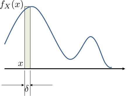
At this point you can see why we call PDF a density, or density function, because each value $f_X(x)$ is the probability per unit length. If we want to calculate the probability of $x \le X \le x + \delta$, for example, then according to our definition, we have

\Pb[x \le X \le x+\delta] = \int_{x}^{x+\delta} f_X(x) \;dx \approx f_X(x) \cdot \delta.

Therefore, the probability of $\Pb[x \le X \le x+\delta]$ can be regarded as the “per unit length” density $f_X(x)$ multiplied with the “length” $\delta$. As $\delta \rightarrow 0$, we can see that $\Pb[X=x] = 0$. See Figure 4.3 for an illustration.

**Figure 4.3.** The probability $\Pb[x \le X \le x + \delta]$ can be approximated by the density $f_X(x)$ multiplied by the length $\delta$.

Why are PDFs called a {density

function?}

sep0ex
Because $f_X(x)$ is the probability per unit length.
You need to integrate $f_X(x)$ to obtain a probability.

Example 4.4

Consider a random variable $X$ with PDF $f_X(x) = \frac{1}{2\sqrt{x}}$ for any $0 < x \le 1$, and is 0 otherwise. We can show that $f_X(x) \rightarrow \infty$ as $x \rightarrow 0$. However, $f_X(x)$ remains a valid PDF because

\begin{aligned} \int_{-\infty}^{\infty} f_X(x) \;dx = \int_0^1 \frac{1}{2\sqrt{x}} \;dx = \sqrt{x}\bigg|_0^1 = 1. \end{aligned}

Remark. Since isolated points have zero measure in the continuous space, the probability of an open interval $(a,b)$ is the same as the probability of a closed interval:

\begin{aligned} \Pb[[a,b]] = \Pb[(a,b)] = \Pb[(a,b]] = \Pb[[a,b)]. \end{aligned}

The exception is that when the PDF of $f_X(x)$ has a delta function at $a$ or $b$. In this case, the probability measure at $a$ or $b$ will be non-zero. We will discuss this when we talk about the CDFs.

Practice Exercise 4.2

Let $f_X(x) = c(1-x^2)$ for $-1 \le x \le 1$, and 0 otherwise. Find the constant $c$.

Solution

Since $\int_{\Omega} f_X(x) \;dx = 1$, it follows that

\begin{aligned} \int_{\Omega} f_X(x) \;dx = \int_{-1}^{1} c(1-x^2) \;dx = \frac{4c}{3} \; \Rightarrow \; c = 3/4. \end{aligned}

Practice Exercise 4.3

Let $f_X(x) = x^2$ for $|x| \le a$, and 0 otherwise. Find $a$.

Solution

Note that $$\int_{\Omega} f_X(x) \;dx = \int_{-a}^a x^2 \;dx = \frac{x^3}{3} \bigg|_{-a}^{a} = \frac{2a^3}{3}.$$ Setting $\frac{2a^3}{3} = 1$ yields $a = \sqrt[3]{\frac{3}{2}}$.

4.1.3Connecting with the PMF

The probability density function is more general than the probability mass function. To see this, consider a discrete random variable $X$ with a PMF $p_X(x)$. Because $p_X$ is defined on a countable set $\Omega$, we can write it as a train of delta functions and define a corresponding PDF:

f_X(x) = \sum_{x_k \in \Omega} p_X(x_k)\;\delta(x - x_k).

Example 4.5

If $X$ is a Bernoulli random variable with PMF $p_X(1) = p$ and $p_X(0) = 1-p$, then the corresponding PDF can be written as

\begin{aligned} f_X(x) = p\;\delta(x-1) + (1-p)\;\delta(x-0). \end{aligned}

Example 4.6

If $X$ is a binomial random variable with PMF $p_X(k) = {n \choose k} p^k (1-p)^{n-k}$, then the corresponding PDF can be written as

\begin{aligned} f_X(x) &= \sum_{k=0}^{n} p_X(k) \; \delta(x-k) \\ &= \sum_{k=0}^{n} {n \choose k} p^k (1-p)^{n-k} \; \delta(x-k). \end{aligned}

Strictly speaking, delta functions are not really functions. They are defined through integrations. They satisfy the properties that $\delta(x-x_k) = \infty$ if $x = x_k$, $\delta(x-x_k) = 0$ if $x \not= x_k$, and $$\int_{x_k-\epsilon}^{x_k+\epsilon} \delta(x-x_k) \;dx = 1,$$ for any $\epsilon > 0$. Suppose we ignore the fact that delta functions are not functions and merely treat them as ordinary functions with some interesting properties. In this case, we can imagine that for every probability mass $p_X(x_k)$, there exists an interval $[a,b]$ such that there is one and only one state $x_k$ that lies in $[a,b]$, as shown in Figure 4.4.

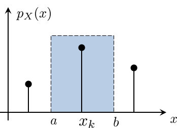
**Figure 4.4.** We can view a PMF as a train of impulses. When computing the probability $X = x_k$, we integrate the PMF over the interval $[a,b]$.

If we want to calculate the probability of obtaining $X = x_k$, we can show that

\begin{aligned} \Pb[X = x_k] &\overset{(a)}{=} \Pb[a \le X \le b] \\ &= \int_{a}^{b} f_X(x) \;dx \\ &\overset{(b)}{=} \int_a^b p_X(x_k) \;\delta(x-x_k) \;dx \\ &\overset{(c)}{=} p_X(x_k) \underset{=1}{\underbrace{\int_{a}^{b}\delta(x-x_k) \;dx}} = p_X(x_k). \end{aligned}

Here, step $(a)$ holds because within $[a,b]$, there is no other event besides $X = x_k$. Step $(b)$ is just the definition of our $f_X(x)$ (inside the interval $[a,b]$). Step $(c)$ shows that the delta function integrates to 1, thus leaving the probability mass $p_X(x_k)$ as the final result. Let us look at an example and then comment on this intuition.

Example 4.7

Let $X$ be a discrete random variable with PMF

p_X(k) = \frac{1}{2^k}, \quad\quad k = 1,2,\ldots

The continuous representation of the PMF can be written as

\begin{aligned} f_X(x) &= \sum_{k = 1}^\infty p_X(k)\; \delta(x - k) = \sum_{k = 1}^\infty \left(\frac{1}{2^k}\right) \delta(x - k). \end{aligned}

Suppose we want to compute the probability $\Pb[1 \le X \le 2]$. This can be computed as

\begin{aligned} \Pb[1 \le X \le 2] &= \int_{1}^2 f_X(x) \;dx = \int_{1}^2 \sum_{k = 1}^\infty \left(\frac{1}{2^k}\right) \delta(x - k) \;dx \\ &= \int_{1}^2 \left\{\frac{1}{2} \delta(x - 1) + \frac{1}{4} \delta(x - 2) + \cdots \right\} \;dx \\ &= \frac{1}{2} \underset{=1}{\underbrace{\int_{1}^2 \delta(x-1)\;dx}} + \frac{1}{4} \underset{=1}{\underbrace{\int_{1}^2 \delta(x-2)\;dx}} \\ &\qquad + \frac{1}{8} \underset{=0}{\underbrace{\int_{1}^2 \delta(x-3)\;dx}} + \underset{=0}{\underbrace{\cdots}} \\ &= \frac{1}{2} + \frac{1}{4} = \frac{3}{4}. \end{aligned}

However, if we want to compute the probability $\Pb[1 < X \le 2]$, then the integration limit will not include the number 1 and so the delta function will remain 0. Thus,

\begin{aligned} \Pb[1 < X \le 2] &= \int_{1^+}^2 f_X(x) \;dx \\ &= \frac{1}{2} \underset{=0}{\underbrace{\int_{1^+}^2 \delta(x-1)\;dx}} + \frac{1}{4} \underset{=1}{\underbrace{\int_{1^+}^2 \delta(x-2)\;dx}} = \frac{1}{4}. \end{aligned}

Closing remark. To summarize, we see that a PMF can be “regarded” as a PDF. We are careful to put a quotation around “regarded” because PMF and PDF are defined for different events. A PMF uses a discrete measure (i.e., a counter) for countable events, whereas a PDF uses a continuous measure (i.e., integration) for continuous events. The way we link the two is by using the delta functions. Using the delta functions is valid, but the argument we provide here is intuitive rather than rigorous. It is not rigorous because the integration we use is still the Riemann-Stieltjes integration, which does not handle delta functions. Therefore, while you can treat a discrete PDF as a train of delta functions, it is important to remember the limitations of the integrations we use.