eBook › Chapter 5 · Joint Distributions

Section 5.1

Joint PMF and Joint PDF

Probability is a measure of the size of a set. This principle applies to discrete random variables, continuous random variables, single random variables, and multiple random variables. In situations with a pair of random variables, the measure should be applied to the coordinate $(X,Y)$ represented by the random variables $X$ and $Y$. Consequently, when measuring the probability, we either count these coordinates or integrate the area covered by these coordinates. In this section, we formalize this notion of measuring 2D events.

5.1.1Probability measure in 2D

Consider two random variables $X$ and $Y$. Let the sample space of $X$ and $Y$ be $\Omega_X$ and $\Omega_Y$, respectively. Define the Cartesian product of $\Omega_X$ and $\Omega_Y$ as $\Omega_X \times \Omega_Y = \{(x,y) \;|\; x \in \Omega_X \;\text{and}\; y \in \Omega_Y\}$. That is, $\Omega_X \times \Omega_Y$ contains all possible pairs $(X,Y)$.

Example 5.1

If $\Omega_X = \{1,2\}$ and $\Omega_Y = \{4,5\}$, then $\Omega_X \times \Omega_Y = \{(1,4),(1,5),$ $(2,4),(2,5)\}.$

Example 5.2

If $\Omega_X = [3,4]$ and $\Omega_Y = [1,2]$, then $\Omega_X \times \Omega_Y =$ a rectangle with two diagonal vertices as $(3,1)$ and $(4,2)$.

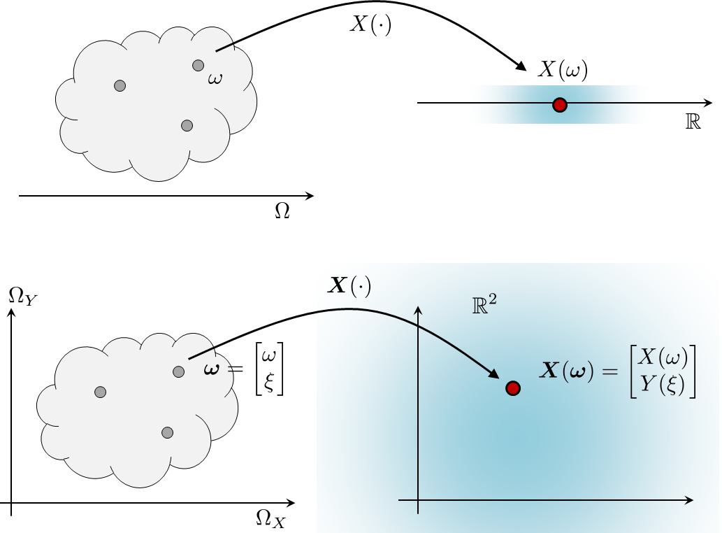
Random variables are mappings from the sample space to the real line. If $\omega \in \Omega_X$ is mapped to $X(\omega) \in \R$, and $\xi \in \Omega_Y$ is mapped to $Y(\xi) \in \R$, then a coordinate $\vomega = (\omega,\xi)$ in the sample space $\Omega_X \times \Omega_Y$ should be mapped to a coordinate $(X(\omega),Y(\xi))$ in the 2D plane.

\vomega \bydef \begin{bmatrix} \omega\\ \xi \end{bmatrix} \longmapsto \begin{bmatrix} X(\omega)\\ Y(\xi) \end{bmatrix} \bydef \mX(\vomega).

We denote such a vector-to-vector mapping as $\mX(\cdot): \Omega_X \times \Omega_Y \rightarrow \R \times \R$, as illustrated in Figure 5.1.

Therefore, if we have an event $\calA \in \R^2$, the probability that $\calA$ happens is

\begin{aligned} \Pb[\calA] &= \Pb[\{\vomega \;|\; \mX(\vomega) \in \calA\}] \\ &= \Pb\bigg[ \bigg\{ \begin{bmatrix}\omega\\ \xi\end{bmatrix} \;\; \bigg|\;\; \begin{bmatrix}X(\omega)\\ Y(\xi)\end{bmatrix} \in \calA \bigg\} \bigg] \\ &= \Pb\bigg[\bigg\{ \begin{bmatrix}\omega\\ \xi\end{bmatrix} \in \mX^{-1}(\calA) \bigg\}\bigg]\\ &= \Pb[\vomega \in \mX^{-1}(\calA)]. \end{aligned}

In other words, we take the coordinate $\mX(\vomega)$ and find its inverse image $\mX^{-1}(\calA)$. The size of this inverse image $\mX^{-1}(\calA)$ in the sample space $\Omega_X \times \Omega_Y$ is then the probability. We summarize this general principle as follows.

How to measure probability in 2D

For a pair of random variables $\mX = (X,Y)$, the probability of an event $\calA$ is measured in the product space $\Omega_X \times \Omega_Y$ with the size $$\Pb[\{\vomega \;|\; \mX^{-1}(\calA)\}].$$

This definition is quite abstract. To make it more concrete, we will look at discrete and continuous random variables.

5.1.2Discrete random variables

Suppose that the random variables $X$ and $Y$ are discrete. Let $\calA = \{X(\omega) = x, \; Y(\xi) = y\}$ be a discrete event. Then the above definition tells us that the probability of $\calA$ is

\begin{aligned} \Pb[\calA] &= \Pb\bigg[ (\omega, \xi) \;\bigg|\; X(\omega) = x, \;\text{and}\; Y(\xi) = y\bigg] = \underset{\bydef p_{X,Y}(x,y)}{\underbrace{\Pb[X = x \; \text{and} \; Y = y]}}. \end{aligned}

We define this probability as the joint probability mass function (joint PMF) $p_{X,Y}(x,y)$.

Definition 5.1

Let $X$ and $Y$ be two discrete random variables. The joint PMF of $X$ and $Y$ is defined as

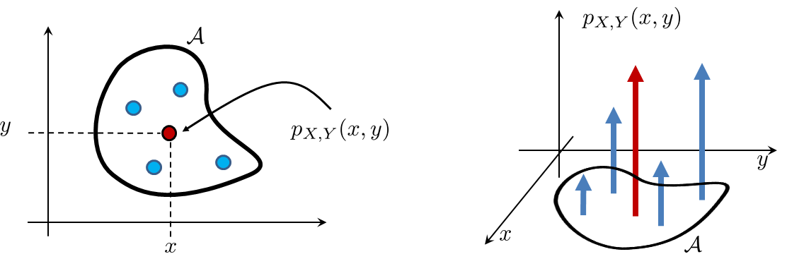
p_{X,Y}(x,y) = \Pb[X =x \; \text{and} \; Y =y] = \Pb\bigg[ (\omega, \xi) \;\bigg|\; X(\omega) = x, \;\text{and}\; Y(\xi) = y \bigg].

We sometimes write the joint PMF as $p_{X,Y}(x,y) = \Pb[X = x,\; Y = y]$. Figure 5.2 shows a graphical portrayal of the joint PMF. In a nutshell, $p_{X,Y}(x,y)$ can be considered as a 2D extension of a single variable PMF. The probabilities are still represented by the impulses, but the domain of these impulses is now a 2D plane. If we have an event $\calA$, then the size of the event is

\Pb[\calA] = \sum_{(x,y) \in \calA} p_{X,Y}(x,y).

Example 5.3

Let $X$ be a coin flip, $Y$ be a die. The sample space of $X$ is $\{0,1\}$, whereas the sample space of $Y$ is $\{1,2,3,4,5,6\}$. The joint PMF, according to our definition, is the probability $\Pb[X = x \text{ and } Y = y]$, where $x$ takes a binary state and $Y$ takes one of the 6 states. The following table summarizes all the 12 states of the joint distribution.

			Y
	1	2	3	4	5	6
X = 0	$\frac{1}{12}$	$\frac{1}{12}$	$\frac{1}{12}$	$\frac{1}{12}$	$\frac{1}{12}$	$\frac{1}{12}$
X = 1	$\frac{1}{12}$	$\frac{1}{12}$	$\frac{1}{12}$	$\frac{1}{12}$	$\frac{1}{12}$	$\frac{1}{12}$

In this table, since there are 12 coordinates, and each coordinate has an equal chance of appearing, the probability for each coordinate becomes $1/12$. Therefore, the joint PMF of $X$ and $Y$ is

p_{X,Y}(x,y) = \frac{1}{12}, \quad x = 0,1, \quad y = 1,2,3,4,5,6.

In this example, we observe that if $X$ and $Y$ are not interacting with each other (formally, independent), the joint PMF is the product of the two individual probabilities.

Example 5.4

In the previous example, if we define $\calA = \{X+Y = 3\}$, the probability $\Pb[\calA]$ is

\begin{aligned} \Pb[\calA] &= \sum_{(x,y)\in \calA} p_{X,Y}(x,y) = p_{X,Y}(0,3) + p_{X,Y}(1,2) \\ &= \frac{2}{12}. \end{aligned}

If $\calB = \{\min(X,Y) = 1\}$, the probability $\Pb[\calB]$ is

\begin{aligned} \Pb[\calB] &= \sum_{(x,y)\in \calB} p_{X,Y}(x,y) \\ &= p_{X,Y}(1,1) + p_{X,Y}(1,2) + p_{X,Y}(1,3) \\ &\qquad\qquad + p_{X,Y}(1,4) + p_{X,Y}(1,5) + p_{X,Y}(1,6) \\ &= \frac{6}{12}. \end{aligned}

5.1.3Continuous random variables

The continuous version of the joint PMF is called the joint probability density function (joint PDF), denoted by $f_{X,Y}(x,y)$. A joint PDF is analogous to a joint PMF. For example, integrating it will give us the probability.

Definition 5.2

Let $X$ and $Y$ be two continuous random variables. The joint PDF of $X$ and $Y$ is a function $f_{X,Y}(x,y)$ that can be integrated to yield a probability

\Pb[ \calA ] = \int_{\calA} f_{X,Y}(x,y) \;dx\;dy,

for any event $\calA \subseteq \Omega_X \times \Omega_Y$.

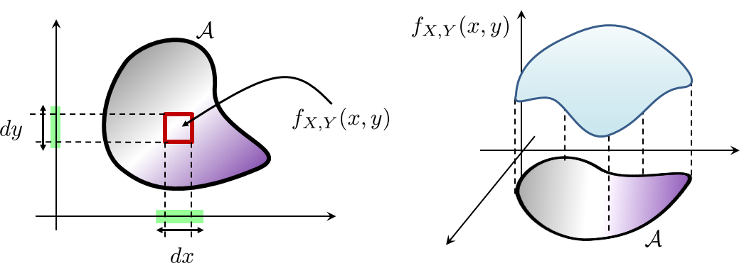
Pictorially, we can view $f_{X,Y}$ as a 2D function where the height at a coordinate $(x,y)$ is $f_{X,Y}(x,y)$, as can be seen from Figure 5.3. To compute the probability that $(X,Y) \in \calA$, we integrate the function $f_{X,Y}$ with respect to the area covered by the set $\calA$. For example, if the set $\calA$ is a rectangular box $\calA = [a,b] \times [c,d]$, then the integration becomes

\begin{aligned} \Pb[\calA] &= \Pb[ a\le X\le b, \;\; c \le Y \le d ] \\ &= \int_c^d \int_a^b f_{X,Y}(x,y) \;dx\;dy. \end{aligned}

Example 5.5

Consider a uniform joint PDF $f_{X,Y}(x,y)$ defined on $[0,2]^2$ with $f_{X,Y}(x,y) = \frac{1}{4}$. Let $\calA = [a,b] \times [c,d]$. Find $\Pb[\calA]$.

Solution

\begin{aligned} \Pb[\calA] &= \Pb[a \le X \le b, \;\; c \le Y \le d]\\ &= \int_{c}^{d} \int_{a}^{b} f_{X,Y}(x,y) \;dx\;dy = \int_{c}^{d} \int_{a}^{b} \frac{1}{4} \;dx\;dy = \frac{(d-c)(b-a)}{4}. \end{aligned}

Practice Exercise 5.1

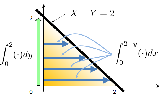
In the previous example, let $\calB = \{X + Y \le 2\}$. Find $\Pb[\calB]$.

Solution

\begin{aligned} \Pb[\calB] &= \int_{\calB} f_{X,Y}(x,y) \;dx\;dy\\ &= \int_{0}^{2} \int_{0}^{2-y} f_{X,Y}(x,y) \;dx\;dy\\ &= \int_{0}^{2} \int_{0}^{2-y} \frac{1}{4} \;dx\;dy \\ &= \int_{0}^{2} \frac{2-y}{4} \;dy = \frac{1}{2}. \end{aligned}

Here, the limits of the integration can be determined from Figure 5.4. The inner integration (with respect to $x$) should start from 0 and end at $2-y$, which is the line defining the set $x+y\le 2$. Since the inner integration is performed for every $y$, we need to enumerate all the possible $y$'s to complete the outer integration. This leads to the outer limit from 0 to 2.

5.1.4Normalization

The normalization property of a two-dimensional PMF and PDF is the property that, when we enumerate all outcomes of the sample space, we obtain 1.

Theorem 5.1

Let $\Omega = \Omega_X \times \Omega_Y$. All joint PMFs and joint PDFs satisfy

\sum_{(x,y) \in \Omega} p_{X,Y}(x,y) = 1 \quad\mbox{or}\quad \int_{\Omega} f_{X,Y}(x,y)\;dx\;dy = 1.

Example 5.6

Consider a joint uniform PDF defined in the shaded area $[0,3]\times[0,3]$ with PDF defined below. Find the constant $c$.

\begin{aligned} f_{X,Y}(x,y) = \begin{cases} c &\quad\mbox{if } (x,y) \in [0,3]\times[0,3],\\ 0 &\quad\mbox{otherwise}. \end{cases} \end{aligned}

Solution

To find the constant $c$, we note that

\begin{aligned} 1 &= \int_{0}^3 \int_{0}^3 f_{X,Y}(x,y)\;dx\;dy \\ &= \int_{0}^3 \int_{0}^3 c \;dx\;dy = 9c . \end{aligned}

Equating the two sides gives us $c = \frac{1}{9}$.

Practice Exercise 5.2

Consider a joint PDF

f_{X,Y}(x,y) = \begin{cases} ce^{-x}e^{-y} &\qquad 0 \le y \le x < \infty,\\ 0 &\qquad \text{otherwise}. \end{cases}

Find the constant $c$. Tip: Consider the area of integration as shown in Figure 5.5.

Solution

There are two ways to take the integration shown in Figure 5.5. We choose the inner integration w.r.t. $y$ first.

\begin{aligned} \int_{\Omega} f_{X,Y}(x,y)\;dx\;dy &= \int_{0}^{\infty} \int_{0}^{x} ce^{-x}e^{-y} \;dy \;dx \\ &= \int_0^{\infty} ce^{-x}(1-e^{-x}) \;dx \\ &= \frac{c}{2}. \end{aligned}

Therefore, $c = 2$.

**Figure 5.5.** To integrate the probability $\Pb[0 \le Y \le X]$, we perform a 2D integration over a triangle. The two subfigures show the two ways of integrating the triangle. [Left] $\int \;dx$ first, and then $\int \;dy$. [Right] $\int \;dy$ first, and then $\int \;dx$.

5.1.5Marginal PMF and marginal PDF

If we only sum / integrate for one random variable, we obtain the PMF / PDF of the other random variable. The resulting PMF / PDF is called the marginal PMF / PDF.

Definition 5.3

The marginal PMF is defined as

p_X(x) = \sum_{y \in \Omega_Y} p_{X,Y}(x,y) \quad\mbox{and}\quad p_Y(y) = \sum_{x\in \Omega_X} p_{X,Y}(x,y),

and the marginal PDF is defined as

f_X(x) = \int_{\Omega_Y} f_{X,Y}(x,y)\;dy \quad\mbox{and}\quad f_Y(y) = \int_{\Omega_X} f_{X,Y}(x,y)\;dx.

Since $f_{X,Y}(x,y)$ is a two-dimensional function, when integrating over $y$ from $-\infty$ to $\infty$, we project $f_{X,Y}(x,y)$ onto the $x$-axis. Therefore, the resulting function depends on $x$ only.

Example 5.7

Consider the joint PDF $f_{X,Y}(x,y) = \frac{1}{4}$ shown below. Find the marginal PDFs.

Solution

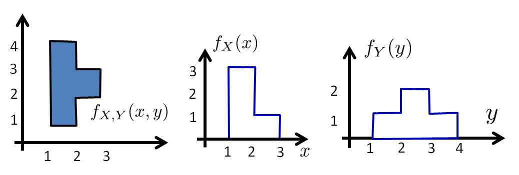
If we integrate over $x$ and $y$, we have

\begin{aligned} f_{X}(x) = \begin{cases} 3/4, &\quad\mbox{if } 1 < x \le 2,\\ 1/4, &\quad\mbox{if } 2 < x \le 3,\\ 0, &\quad\mbox{otherwise}. \end{cases} \quad \mbox{and} \quad f_Y(y) = \begin{cases} 1/4, &\quad\mbox{if } 1 < y \le 2,\\ 1/2, &\quad\mbox{if } 2 < y \le 3,\\ 1/4, &\quad\mbox{if } 3 < y \le 4,\\ 0, &\quad\mbox{otherwise}. \end{cases} \end{aligned}

So the marginal PDFs are the projection of the joint PDFs onto the $x$- and $y$-axes.

Practice Exercise 5.3

A joint Gaussian random variable $(X,Y)$ has a joint PDF given by

f_{X,Y}(x,y) = \frac{1}{2\pi \sigma^2} \exp\left\{-\frac{((x-\mu_X)^2 + (y-\mu_Y)^2)}{2\sigma^2}\right\}.

Find the marginal PDFs $f_X(x)$ and $f_Y(y)$.

Solution

\begin{aligned} f_X(x) &= \int_{-\infty}^{\infty} f_{X,Y}(x,y) \;dy = \int_{-\infty}^{\infty} \frac{1}{2\pi \sigma^2} \exp\left\{-\frac{((x-\mu_X)^2 + (y-\mu_Y)^2)}{2\sigma^2}\right\} \;dy \\ &= \frac{1}{\sqrt{2\pi \sigma^2}} \exp\left\{-\frac{(x-\mu_X)^2}{2\sigma^2}\right\} \cdot \int_{-\infty}^{\infty} \frac{1}{\sqrt{2\pi \sigma^2}} \exp\left\{-\frac{(y-\mu_Y)^2}{2\sigma^2}\right\} \;dy. \end{aligned}

Recognizing that the last integral is equal to unity because it integrates a Gaussian PDF over the real line, it follows that

\begin{aligned} f_X(x) = \frac{1}{\sqrt{2\pi \sigma^2}} \exp\left\{-\frac{(x-\mu_X)^2}{2\sigma^2}\right\}. \end{aligned}

Similarly, we have $$f_Y(y) = \frac{1}{\sqrt{2\pi \sigma^2}} \exp\left\{-\frac{(y-\mu_Y)^2}{2\sigma^2}\right\}.$$

5.1.6Independent random variables

Two random variables are said to be independent if and only if the joint PMF or PDF can be factorized as a product of the marginal PMF / PDFs.

Definition 5.4

Random variables $X$ and $Y$ are independent if and only if

\begin{aligned} p_{X,Y}(x,y) = p_X(x)\;p_Y(y), \quad\mbox{or}\quad f_{X,Y}(x,y) = f_X(x)\;f_Y(y). \end{aligned}

This definition is consistent with the definition of independence of two events. Recall that two events $A$ and $B$ are independent if and only if $\Pb[A \cap B] = \Pb[A]\Pb[B]$. Letting $A = \{X = x\}$ and $B = \{Y = y\}$, we see that if $A$ and $B$ are independent then $\Pb[X = x \cap Y = y]$ is the product $\Pb[X = x]\Pb[Y = y]$. This is precisely the relationship $p_{X,Y}(x,y) = p_X(x)\;p_Y(y)$.

Example 5.8

Consider two random variables with a joint PDF given by

f_{X,Y}(x,y) = \frac{1}{2\pi \sigma^2} \exp\left\{-\frac{(x-\mu_X)^2 + (y-\mu_Y)^2}{2\sigma^2}\right\}.

Are $X$ and $Y$ independent?

Solution

We know that

f_{X,Y}(x,y) = \underset{f_X(x)}{\underbrace{\frac{1}{\sqrt{2\pi} \sigma} \exp\left\{-\frac{(x-\mu_X)^2}{2\sigma^2}\right\}}} \times \underset{f_Y(y)}{\underbrace{\frac{1}{\sqrt{2\pi} \sigma} \exp\left\{-\frac{(y-\mu_Y)^2}{2\sigma^2}\right\}}}.

Therefore, the random variables $X$ and $Y$ are independent.

Practice Exercise 5.4

Let $X$ be a coin and $Y$ be a die. Then the joint PMF is given by the table below.

			Y
	1	2	3	4	5	6
X = 0	$\frac{1}{12}$	$\frac{1}{12}$	$\frac{1}{12}$	$\frac{1}{12}$	$\frac{1}{12}$	$\frac{1}{12}$
X = 1	$\frac{1}{12}$	$\frac{1}{12}$	$\frac{1}{12}$	$\frac{1}{12}$	$\frac{1}{12}$	$\frac{1}{12}$

Are $X$ and $Y$ independent?

Solution

For any $x$ and $y$, we have that

p_{X,Y}(x,y) = \frac{1}{12} = \underset{p_X(x)}{\underbrace{\frac{1}{2}}} \times \underset{p_Y(y)}{\underbrace{\frac{1}{6}}}.

Therefore, the random variables $X$ and $Y$ are independent.

Example 5.9

Consider two random variables $X$ and $Y$ with a joint PDF given by (We use the notation “$\propto$” to denote “proportional to”. It implies that the normalization constant is omitted.)

\begin{aligned} f_{X,Y}(x,y) \propto \exp\left\{-(x-y)^2\right\} &= \exp\left\{-x^2 + 2xy - y^2\right\}\\ &= \underset{f_X(x)}{\underbrace{\exp\left\{-x^2\right\}}} \;\; \underset{\text{extra term}}{\underbrace{\exp\left\{2xy\right\}}} \;\; \underset{f_Y(y)}{\underbrace{\exp\left\{-y^2\right\}}}. \end{aligned}

This PDF cannot be factorized into a product of two marginal PDFs. Therefore, the random variables are dependent.

We can extrapolate the definition of independence to multiple random variables. If there are many random variables $X_1,X_2,\ldots,X_N$, they will have a joint PDF

f_{X_1,\ldots,X_N}(x_1,\ldots,x_N).

If these random variables $X_1,X_2,\ldots,X_N$ are independent, then the joint PDF can be factorized as

\begin{aligned} f_{X_1,\ldots,X_N}(x_1,\ldots,x_N) &= f_{X_1}(x_1) \cdot f_{X_2}(x_2) \cdots f_{X_N}(x_N) \\ &= \prod_{n=1}^N f_{X_n}(x_n). \end{aligned}

This gives us the definition of independence for $N$ random variables.

Definition 5.5

A sequence of random variables $X_1, \ldots, X_N$ is independent if and only if their joint PDF (or joint PMF) can be factorized.

f_{X_1,\ldots,X_N}(x_1,\ldots,x_N) = \prod_{n=1}^N f_{X_n}(x_n).

Example 5.10

Throw a die 4 times. Let $X_1$, $X_2$, $X_3$ and $X_4$ be the outcomes. Then, since these four throws are independent, the probability mass function of any quadruple $(x_1,x_2,x_3,x_4)$ is

p_{X_1,X_2,X_3,X_4}(x_1,x_2,x_3,x_4) = p_{X_1}(x_1)\;p_{X_2}(x_2)\;p_{X_3}(x_3)\;p_{X_4}(x_4).

For example, the probability of getting $(1,5,2,6)$ is

p_{X_1,X_2,X_3,X_4}(1,5,2,6) = p_{X_1}(1)\;p_{X_2}(5)\;p_{X_3}(2)\;p_{X_4}(6) = \left(\frac{1}{6}\right)^4.

The example above demonstrates an interesting phenomenon. If the $N$ random variables are independent, and if they all have the same distribution, then the joint PDF/PMF is just one of the individual PDFs taken to the power $N$. Random variables satisfying this property are known as independent and identically distributed random variables.

Definition 5.6 (Independent and Identically Distributed (i.i.d.))

A collection of random variables $X_1,\ldots,X_N$ is called independent and identically distributed (i.i.d.) if

sep0ex
All $X_1,\ldots,X_N$ are independent; and
All $X_1,\ldots,X_N$ have the same distribution, i.e., $f_{X_1}(x) = \cdots = f_{X_N}(x)$.

If $X_1,\ldots,X_N$ are i.i.d., we have that

f_{X_1,\ldots,X_N}(x_1,\ldots,x_N) = \prod_{n=1}^N f_{X_1}(x_n),

where the particular choice of $X_1$ is unimportant because $f_{X_1}(x) = \cdots = f_{X_N}(x)$.

Why is i.i.d. so important?

sep0em
If a set of random variables are i.i.d., then the joint PDF can be written as a product of PDFs.
Integrating a joint PDF is difficult. Integrating a product of PDFs is much easier.

Example 5.11

Let $X_1,X_2,\ldots,X_N$ be a sequence of i.i.d. Gaussian random variables where each $X_i$ has a PDF

f_{X_i}(x) = \frac{1}{\sqrt{2\pi}}\exp\left\{-\frac{x^2}{2}\right\}.

The joint PDF of $X_1,X_2,\ldots,X_N$ is

\begin{aligned} f_{X_1,\ldots,X_N}(x_1,\ldots,x_N) &= \prod_{i=1}^N \left\{\frac{1}{\sqrt{2\pi}}\exp\left\{-\frac{x_i^2}{2}\right\}\right\} \\ &= \left(\frac{1}{\sqrt{2\pi}}\right)^N \exp\left\{-\sum_{i=1}^N \frac{x_i^2}{2}\right\}, \end{aligned}

which is a function depending not on the individual values of $x_1,x_2,\ldots,x_N$ but on the sum $\sum_{i=1}^N x_i^2$. So we have “compressed” an $N$-dimensional function into a 1D function.

Example 5.12

Let $\theta$ be a deterministic number that was sent through a noisy channel. We model the noise as an additive Gaussian random variable with mean $0$ and variance $\sigma^2$. Supposing we have observed measurements $X_i = \theta + W_i$, for $i = 1,\ldots,N$, where $W_i \sim \text{Gaussian}(0,\sigma^2)$, then the PDF of each $X_i$ is $$f_{X_i}(x) = \frac{1}{\sqrt{2\pi\sigma^2}}\exp\left\{-\frac{(x-\theta)^2}{2\sigma^2}\right\}.$$ Thus the joint PDF of $(X_1,X_2,\ldots,X_N)$ is

\begin{aligned} f_{X_1,\ldots,X_N}(x_1,\ldots,x_N) &= \prod_{i=1}^N \left\{\frac{1}{\sqrt{2\pi\sigma^2}}\exp\left\{-\frac{(x_i-\theta)^2}{2\sigma^2}\right\}\right\} \\ &= \left(\frac{1}{\sqrt{2\pi\sigma^2}}\right)^N \exp\left\{-\sum_{i=1}^N \frac{(x_i-\theta)^2}{2\sigma^2}\right\}. \end{aligned}

Essentially, this joint PDF tells us the probability density of seeing sample data $x_1,\ldots,x_N$.

5.1.7Joint CDF

We now introduce the cumulative distribution function (CDF) for multiple variables.

Definition 5.7

Let $X$ and $Y$ be two random variables. The joint CDF of $X$ and $Y$ is the function $F_{X,Y}(x,y)$ such that

F_{X,Y}(x,y) = \Pb[X \le x \;\cap\; Y \le y].

This definition can be more explicitly written as follows.

Definition 5.8

If $X$ and $Y$ are discrete, then

F_{X,Y}(x,y) = \sum_{y' \le y} \sum_{x' \le x} p_{X,Y}(x',y').

If $X$ and $Y$ are continuous, then

F_{X,Y}(x,y) = \int_{-\infty}^{y} \int_{-\infty}^{x} f_{X,Y}(x',y')\;dx'\;dy'.

If the two random variables are independent, then we have

F_{X,Y}(x,y) = \int_{-\infty}^{x} f_{X}(x')\;dx' \int_{-\infty}^{y} f_Y(y')\;dy' = F_X(x) F_Y(y).

Example 5.13

Let $X$ and $Y$ be two independent uniform random variables\ $\text{Uniform}(0,1)$. Find the joint CDF.

Solution

\begin{aligned} F_{X,Y}(x,y) &= \int_{0}^{x} f_X(x')\;dx' \int_{0}^{y} f_Y(y')\;dy' = \int_{0}^{x} 1 \;dx' \int_{0}^{y} 1 \;dy' = xy. \end{aligned}

Practice Exercise 5.5

Let $X$ and $Y$ be two independent Gaussian random variables $\text{Gaussian}(\mu,\sigma^2)$. Find the joint CDF.

Solution

Let $\Phi(\cdot)$ be the CDF of the standard Gaussian.

\begin{aligned} F_{X,Y}(x,y) &= F_X(x)F_Y(y) \\ &= \int_{-\infty}^{x} f_X(x')\;dx' \int_{-\infty}^{y} f_Y(y')\;dy' = \Phi\left(\frac{x-\mu}{\sigma}\right)\Phi\left(\frac{y-\mu}{\sigma}\right). \end{aligned}

Here are a few properties of the CDF:

\begin{aligned} F_{X,Y}(x,-\infty) &= \int_{-\infty}^{-\infty} \int_{-\infty}^{x} f_{X,Y}(x',y')\;dx'\;dy' = \int_{-\infty}^{x} 0 \;dx' = 0,\\ F_{X,Y}(-\infty,y) &= \int_{-\infty}^{y} \int_{-\infty}^{-\infty} f_{X,Y}(x',y')\;dx'\;dy' = \int_{-\infty}^{y} 0 \;dy' = 0,\\ F_{X,Y}(-\infty,-\infty) &= \int_{-\infty}^{-\infty} \int_{-\infty}^{-\infty} f_{X,Y}(x',y')\;dx'\;dy' = 0,\\ F_{X,Y}(\infty,\infty) &= \int_{-\infty}^{\infty} \int_{-\infty}^{\infty} f_{X,Y}(x',y')\;dx'\;dy' = 1. \end{aligned}

In addition, we can obtain the marginal CDF as follows.

Proposition 5.1

Let $X$ and $Y$ be two random variables. The marginal CDF is

\begin{aligned} F_X(x) &= F_{X,Y}(x,\infty),\\ F_Y(y) &= F_{X,Y}(\infty,y). \end{aligned}

Proof. We prove only the first case. The second case is similar.

\begin{aligned} F_{X,Y}(x,\infty) &= \int_{-\infty}^{x} \int_{-\infty}^{\infty} f_{X,Y}(x',y')\;dy' \;dx' = \int_{-\infty}^{x} f_X(x') \;dx' = F_X(x). \end{aligned}

■

By the fundamental theorem of calculus, we can derive the PDF from the CDF.

Definition 5.9

Let $F_{X,Y}(x,y)$ be the joint CDF of $X$ and $Y$. Then, the joint PDF is

\begin{aligned} f_{X,Y}(x,y) = \frac{\partial^2}{\partial y \; \partial x} F_{X,Y}(x,y). \end{aligned}

The order of the partial derivatives can be switched, yielding a symmetric result:

\begin{aligned} f_{X,Y}(x,y) = \frac{\partial^2}{\partial x \; \partial y } F_{X,Y}(x,y). \end{aligned}

Example 5.14

Let $X$ and $Y$ be two uniform random variables with joint CDF $F_{X,Y}(x,y) = xy$ for $0 \le x \le 1$ and $0 \le y \le 1$. Find the joint PDF.

Solution

\begin{aligned} f_{X,Y}(x,y) &= \frac{\partial^2}{\partial x \partial y } F_{X,Y}(x,y) = \frac{\partial^2}{\partial x \partial y } xy = 1, \end{aligned}

which is consistent with the definition of a joint uniform random variable.

Practice Exercise 5.6

Let $X$ and $Y$ be two exponential random variables with joint CDF

F_{X,Y}(x,y) = (1-e^{-\lambda x})(1-e^{-\lambda y}), \qquad x \ge 0, \; y \ge 0.

Find the joint PDF.

Solution

\begin{aligned} f_{X,Y}(x,y) = \frac{\partial^2}{\partial x \partial y } F_{X,Y}(x,y) &= \frac{\partial^2}{\partial x \partial y } (1-e^{-\lambda x})(1-e^{-\lambda y}) \\ &= \frac{\partial}{\partial x}\left((1-e^{-\lambda x})(\lambda e^{-\lambda y})\right) = \lambda e^{-\lambda x} \lambda e^{-\lambda y}, \end{aligned}

which is consistent with the definition of a joint exponential random variable.

			Y
	1	2	3	4	5	6
X = 0	\(\frac{1}{12}\)	\(\frac{1}{12}\)	\(\frac{1}{12}\)	\(\frac{1}{12}\)	\(\frac{1}{12}\)	\(\frac{1}{12}\)
X = 1	\(\frac{1}{12}\)	\(\frac{1}{12}\)	\(\frac{1}{12}\)	\(\frac{1}{12}\)	\(\frac{1}{12}\)	\(\frac{1}{12}\)

			Y
	1	2	3	4	5	6
X = 0	\(\frac{1}{12}\)	\(\frac{1}{12}\)	\(\frac{1}{12}\)	\(\frac{1}{12}\)	\(\frac{1}{12}\)	\(\frac{1}{12}\)
X = 1	\(\frac{1}{12}\)	\(\frac{1}{12}\)	\(\frac{1}{12}\)	\(\frac{1}{12}\)	\(\frac{1}{12}\)	\(\frac{1}{12}\)