eBook › Chapter 6 · Sample Statistics

Section 6.2

Probability Inequalities

Moment-generating functions and characteristic functions are powerful tools for handling the sum of random variables. We now introduce another set of tools, known as the probability inequalities, that allow us to do approximations. We will highlight a few basic probability inequalities in this section.

6.2.1Union bound

The first inequality is the union bound we had introduced when we discussed the axioms of probability. The union bound states the following:

Theorem 6.8 (Union Bound)

Let $A_1,\ldots,A_N$ be a collection of sets. Then

\Pb \left[ \bigcup_{n=1}^N A_n \right] \le \sum_{n=1}^N \Pb[A_n].

Proof. We can prove this by induction. First, if $N = 2$,

\begin{aligned} \Pb[A_1 \cup A_2] = \Pb[A_1] + \Pb[A_2] - \Pb[A_1 \cap A_2] \le \Pb[A_1] + \Pb[A_2], \end{aligned}

because $\Pb[A_1 \cap A_2]$ is a probability and so it must be non-negative. Thus we have proved the base case. Assume that the statement is true for $N = K$. We need to prove that the statement is also true for $N = K+1$. To this end, we note that

\begin{aligned} \Pb \left[ \bigcup_{n=1}^{K+1} A_n \right] &= \Pb \left[ \left(\bigcup_{n=1}^{K} A_n\right) \cup A_{K+1} \right]\\ &= \Pb \left[ \bigcup_{n=1}^{K} A_n \right] + \Pb[A_{K+1}] - \Pb \left[ \left(\bigcup_{n=1}^{K} A_n\right) \cap A_{K+1} \right] \\ &\le \Pb \left[ \bigcup_{n=1}^{K} A_n \right] + \Pb[A_{K+1}]. \end{aligned}

Then, according to our hypothesis for $N = K$, it follows that

\begin{aligned} \Pb \left[ \bigcup_{n=1}^{K} A_n \right] \le \sum_{n=1}^K \Pb[A_n]. \end{aligned}

Putting these together,

\begin{aligned} \Pb \left[ \bigcup_{n=1}^{K+1} A_n \right] \le \sum_{n=1}^{K} \Pb[A_n] + \Pb[A_{K+1}] = \sum_{n=1}^{K+1} \Pb[A_n]. \end{aligned}

Therefore, by the principle of induction, we have proved the statement.

■

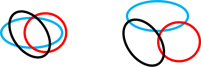
Remark. The tightness of the union bound depends on the amount of overlapping between the events $A_1,\ldots,A_N$, as illustrated in Figure 6.1. If the events are disjoint, the union bound is tight. If the events are overlapping significantly, the union is loose. The idea of the union bound is the principle of divide and conquer. We decompose the system into smaller events for a system of $n$ variables and use the union bound to upper-limit the overall probability. If the probability of each event is small, the union bound tells us that the overall probability of the system will also be small.

Example 6.6

Let $X_1,\ldots,X_N$ be a sequence of i.i.d. random variables with CDF $F_{X_n}(x)$ and let $Z = \min(X_1,\ldots,X_N)$. Find an upper bound on the CDF of $Z$.

Solution

Note that $Z = \min(X_1,\ldots,X_N) \le z$ is equivalent to at least one of the $X_n$'s being less than $z$. Thus, we have that

\begin{aligned} Z = \min(X_1,\ldots,X_N) \le z \;\; \Leftrightarrow \;\; X_1 \le z \cup \cdots \cup X_N \le z. \end{aligned}

Substituting this result into the CDF,

\begin{aligned} F_Z(z) &= \Pb[Z \le z] \\ &= \Pb[\min(X_1,\ldots,X_N) \le z]\\ &= \Pb[X_1 \le z \cup \cdots \cup X_N \le z] \\ &\le \Pb[X_1 \le z] + \cdots + \Pb[ X_N \le z]\\ &= N \cdot F_X(z). \end{aligned}

6.2.2The Cauchy-Schwarz inequality

The second inequality we study here is the Cauchy-Schwarz inequality, which we previously mentioned in Chapter 5. We review it for the sake of completeness.

Theorem 6.9 (Cauchy-Schwarz inequality)

Let $X$ and $Y$ be two random variables. Then

\E[XY]^2 \le \E[X^2] \E[Y^2].

Proof. Let $f(s) = \E[(sX + Y)^2]$ for any real $s$. Then

\begin{aligned} f(s) &= \E[(sX + Y)^2] \\ &= \E[s^2X^2 + 2sXY + Y^2]\\ &= \E[X^2]s^2 + 2\E[XY]s + \E[Y^2]. \end{aligned}

This is a quadratic equation, and $f(s) \ge 0$ for all $s$ because $\E[(sX + Y)^2] \ge 0$.

Recall that for a quadratic equation $\phi(x) = ax^2+bx+c$, if the function $\phi(x) \ge 0$ then $b^2 - 4ac \le 0$. Substituting this result into our problem, we show that

(2\E[XY])^2 - 4\E[X^2]\E[Y^2] \le 0.

This implies that

\E[XY]^2 \le \E[X^2]\E[Y^2],

which completes the proof.

■

Remark. As shown in Chapter 5, the Cauchy-Schwarz inequality is useful in analyzing $\E[XY]$. For example, we can use the Cauchy-Schwarz inequality to prove that the correlation coefficient $\rho$ is bounded between $-1$ and $1$.

6.2.3Jensen's inequality

Our next inequality is Jensen's inequality. To motivate the inequality, we recall that

\Var[X] = \E[X^2] - \E[X]^2.

Since $\Var[X]\ge 0$ for any $X$, it follows that

\underset{=\E[\textcolor{blue}{g}(X)]}{\underbrace{\;\;\E[X^2]\;\;}} \quad \ge \quad \underset{=\textcolor{blue}{g}(\E[X])}{\underbrace{\;\;\E[X]^2\;\;}}.

Jensen's inequality is a generalization of the above result by recognizing that the inequality does not only hold for the function $g(X) = X^2$ but also for any convex function $g$. The theorem is stated as follows:

Theorem 6.10 (Jensen's inequality)

Let $X$ be a random variable, and let $g: \R \rightarrow \R$ be a convex function. Then

\E[g(X)] \ge g(\E[X]).

If the function $g$ is concave, then the inequality sign is flipped: $\E[g(X)] \le g(\E[X])$. The way to remember this result is to remember that $\E[X^2] - \E[X]^2 = \Var[X] \ge 0$.

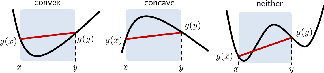
Now, what is a convex function? Informally, a function $g$ is convex if, when we pick any two points on the function and connect them with a straight line, the line will be above the function for that segment. This definition is illustrated in Figure 6.2. Consider an interval $[x,y]$, and the line segment connecting $g(x)$ and $g(y)$. If the function $g(\cdot)$ is convex, then the entire line segment should be above the curve.

**Figure 6.2.** Illustration of a convex function, a concave function, and a function that is neither convex nor concave.

The definition of a convex function essentially follows the above picture:

Definition 6.4

A function $g$ is convex if

g(\lambda x + (1-\lambda)y) \le \lambda g(x) + (1-\lambda) g(y),

for any $0 \le \lambda \le 1$.

Here $\lambda$ represents a “sweeping” constant that goes from $0$ to $1$. When $\lambda = 1$ then $\lambda x + (1-\lambda)y$ simplifies to $x$, and when $\lambda = 0$ then $\lambda x + (1-\lambda)y$ simplifies to $y$.

The definition is easy to understand. The left-hand side $g(\lambda x + (1-\lambda)y)$ is the function evaluated at any points in the interval $[x,y]$. The right-hand side is the red straight line we plotted in Figure 6.2. It connects the two points $g(x)$ and $g(y)$. Convexity means that the red line is entirely above the curve.

For twice-differentiable 1D functions, convexity can be described by the curvature of the function. A function is convex if

g''(x) \ge 0.

This is self-explanatory because if the curvature is non-negative for all $x$, then the slope of $g$ has to keep increasing.

Example 6.7

The following functions are convex or concave:

sep0ex
$g(x) = \log x$ is concave, because $g'(x) = \frac{1}{x}$ and $g''(x) = -\frac{1}{x^2} \le 0$ for all $x$.
$g(x) = x^2$ is convex, because $g'(x) = 2x$ and $g''(x) = 2$ is positive.
$g(x) = e^{-x}$ is convex, because $g'(x) = -e^{-x}$ and $g''(x) = e^{-x} \ge 0$.

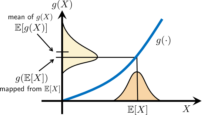
Why is Jensen's inequality valid for a convex function? Consider the illustration in Figure 6.3. Suppose we have a random variable $X$ taking some PDF $f_X(x)$. There is a convex function $g(\cdot)$ that maps the random variable $X$ to $g(X)$. Since $g(\cdot)$ is convex, a PDF like the one we see in Figure 6.3 will become skewed. (You can map the left tail to the new left tail, the peak to the new peak, and the right tail to the new right tail.) As you can see from the figure, the new random variable $g(X)$ has a mean $\E[g(X)]$ that is greater than the mapped old mean $g(\E[X])$. Jensen's inequality captures this phenomenon by stating that $\E[g(X)] \ge g(\E[X])$ for any convex function $g(\cdot)$.

Proving Jensen's inequality is straightforward for a two-state discrete random variable. Define a random variable $X$ with states $x$ and $y$. The probabilities for these two states are $\Pb[X = x] = \lambda$ and $\Pb[X =y] = 1-\lambda$. Then

\E[X] = \sum_{x' \in \{x,y\}} x' p_X(x') = \lambda x + (1-\lambda)y.

Now, let $g(\cdot)$ be a convex function. We know from the expectation that

\E[g(X)] = \sum_{x' \in \{x,y\}} g(x') p_X(x') = g(x)\lambda + (1-\lambda)g(y).

By convexity of the function $g(\cdot)$, it follows that

\underset{=g(\E[X])}{\underbrace{g(\lambda x + (1-\lambda)y)}} \le \underset{=\E[g(X)]}{\underbrace{\lambda g(x) + (1-\lambda) g(y)}},

where in the underbrace we substitute the definitions using the expectation. Therefore, for any two-state discrete random variables, the proof of Jensen's inequality follows directly from the convexity. If the discrete random variable takes more than two states, we can prove the theorem by induction. For continuous random variables, we can prove the theorem using the following approach.

You may skip the proof of Jensen's inequality if this is your first time reading the book.

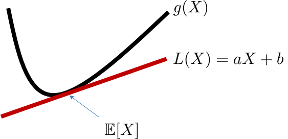
Here we present an alternative proof of Jensen's inequality that does not require proof by induction. The idea is to recognize that if the function $g$ is convex we can find a tangent line $L(X) = aX+b$ at the point $\E[X]$ that is uniformly lower than $g(X)$, i.e., $g(X) \ge L(X)$ for all $X$. Then we can prove the result with a simple geometric argument. Figure 6.4 illustrates this idea.

**Figure 6.4.** Geometric illustration of the proof of Jensen's inequality. Suppose $g(\cdot)$ is a convex function. For any point $X$ on $g(\cdot)$, we can find a tangent line $L(X) = aX+b$. Since the black curve is always above the tangent, it follows that $\E[g(X)] \ge \E[L(X)]$ for any $X$. Also, note that at a particular point $\E[X]$, the black curve and the red line touch, and so we have $L(\E[X]) = g(\E[X])$.

Proof of Jensen's inequality. Consider $L(X)$ as defined above. Since $g$ is convex, $g(X) \ge L(X)$ for all $X$. Therefore,

\begin{aligned} \E[g(X)] &\ge \E[L(X)]\\ &= \E[aX + b] \\ &= a\E[X] + b \\ &= L(\E[X]) = g(\E[X]), \end{aligned}

where the last equality holds because $L$ is a tangent line to $g$ where they meet at $\E[X]$.

■

What are $(a,b)$ in the proof? By Taylor expansion,

\begin{aligned} g(X) &\approx g(\E[X]) + g'(\E[X])(X-\E[X]) \\ &\bydef L(X). \end{aligned}

Therefore, if we want to be precise, then $a = g'(\E[X])$ and $b = g(\E[X]) - g'(\E[X])\E[X]$.

The end of the proof.

Example 6.8

By Jensen's inequality, we have that

sep0ex
(a) $\E[X^2] \ge \E[X]^2$, because $g(x) = x^2$ is convex.
(b) $\E\left[\frac{1}{X}\right] \ge \frac{1}{\E[X]}$, because $g(x) = \frac{1}{x}$ is convex.
(c) $\E[\log X] \le \log \E[X]$, because $g(x) = \log x$ is concave.

6.2.4Markov's inequality

Our next inequality, Markov's inequality, is an elementary inequality that links probability and expectation.

Theorem 6.11 (Markov's inequality)

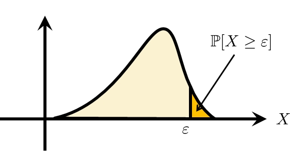
Let $X \ge 0$ be a non-negative random variable. Then, for any $\varepsilon > 0$, we have

\Pb[X \ge \varepsilon] \le \frac{\E[X]}{\varepsilon}.

Markov's inequality concerns the tail of the random variable. As illustrated in Figure 6.5, $\Pb[X \ge \varepsilon]$ measures the probability that the random variable takes a value greater than $\varepsilon$. Markov's inequality asserts that this probability $\Pb[X \ge \varepsilon]$ is upper-bounded by the ratio $\E[X]/\varepsilon$. This result is useful because it relates the probability and the expectation. In many problems the probability $\Pb[X \ge \varepsilon]$ could be difficult to evaluate if the PDF is complicated. The expectation, on the other hand, is usually easier to evaluate.

Proof. Consider $\varepsilon\Pb[X \ge \varepsilon]$. It follows that

\begin{aligned} \varepsilon\Pb[X \ge \varepsilon] = \int_{\varepsilon}^{\infty} \varepsilon \ f_X(x) \;dx \le \int_{\varepsilon}^{\infty} x f_X(x) \;dx, \end{aligned}

where the inequality is valid because for any $x \ge \varepsilon$ the integrand (which is non-negative) will always increase (or at least not decrease). It then follows that

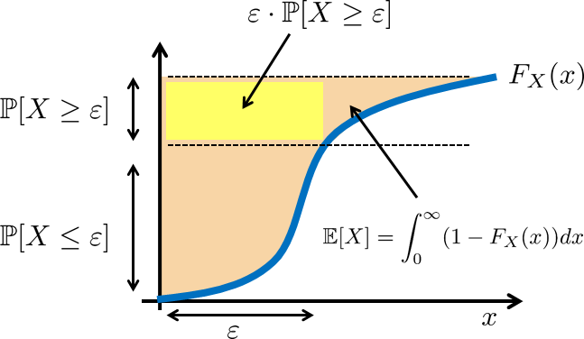
\begin{aligned} \int_{\varepsilon}^{\infty} x f_X(x) \;dx \le \int_{0}^{\infty} x f_X(x) \;dx = \E[X]. \end{aligned}

■

A pictorial interpretation of Markov's inequality is shown in Figure 6.6. For $X > 0$, it is not difficult to show that $\E[X] = \int_0^{\infty} 1-F_X(x) \;dx$. Then, in the CDF plot, we see that $\varepsilon \cdot \Pb[X \ge \varepsilon]$ is a rectangle covering the top left corner. This area is clearly smaller than the area covered by the function $1-F_X(x)$.

Practice Exercise 6.4

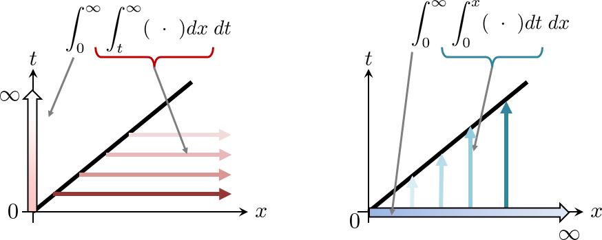
Prove that if $X > 0$, then $\E[X] = \int_0^{\infty} 1-F_X(x) \;dx$.

Solution

We start from the right-hand side:

\begin{aligned} \int_0^{\infty} 1-F_X(x) \;dx &= \int_0^{\infty} 1-\Pb[X \le x] \;dx \\ &= \int_0^{\infty} \Pb[X \ge x] \;dx \\ &= \int_0^{\infty} \int_{x}^{\infty} f_X(t) \; d\textcolor{blue}{t} \; d\textcolor{blue}{x} \\ &= \int_0^{\infty} \int_{0}^{t} f_X(t) \; d\textcolor{blue}{x} \; d\textcolor{blue}{t} \\ &= \int_0^{\infty} t f_X(t) \;dt = \E[X]. \end{aligned}

The change in the integration order is illustrated below.

How tight is Markov's inequality? It is possible to create a random variable such that the equality is met (see Exercise 6.14). However, in general, the estimate provided by the upper bound is not tight. Here is an example.

Practice Exercise 6.5

Let $X \sim \text{Uniform}(0,4)$. Verify Markov's inequality for $\Pb[X \ge 2]$, $\Pb[X \ge 3]$ and $\Pb[X \ge 4]$.

Solution

First, we observe that $\E[X] = 2$. Then

\begin{aligned} \Pb[X \ge 2] = 0.5, &\qquad \frac{\E[X]}{2} = 1,\\ \Pb[X \ge 3] = 0.25, &\qquad \frac{\E[X]}{3} = 0.67,\\ \Pb[X \ge 4] = 0, &\qquad \frac{\E[X]}{4} = 0.5. \end{aligned}

Therefore, although the upper bounds are all valid, they are very loose.

If Markov's inequality is not tight, why is it useful? It turns out that while Markov's inequality is not tight, its variations can be powerful. We will come back to this point when we discuss Chernoff's bound.

6.2.5Chebyshev's inequality

The next inequality is a simple extension of Markov's inequality. The result is known as Chebyshev's inequality.

Theorem 6.12 (Chebyshev's inequality)

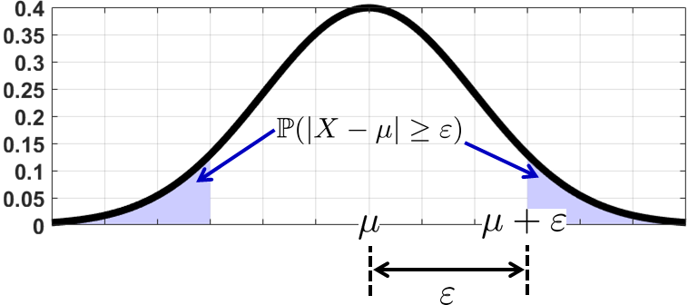
Let $X$ be a random variable with mean $\mu$. Then for any $\varepsilon > 0$ we have

\Pb[|X - \mu| \ge \varepsilon] \le \frac{\Var[X]}{\varepsilon^2}.

The tail measured by Chebyshev's inequality is illustrated in Figure 6.8. Since the event $|X - \mu| \ge \varepsilon$ involves an absolute value, the probability measures the two-sided tail. Chebyshev's inequality states that this tail probability is upper-bounded by $\Var[X]/\varepsilon^2$.

Proof. We apply Markov's inequality to show that

\begin{aligned} \Pb[|X - \mu| \ge \varepsilon] &= \Pb[ (X-\mu)^2\ge \varepsilon^2] \\ &\le \frac{\E[(X-\mu)^2]}{\varepsilon^2} = \frac{\Var[X]}{\varepsilon^2}. \end{aligned}

■

An alternative form of Chebyshev's inequality is obtained by letting $\varepsilon = k\sigma$. In this case, we have

\Pb[|X-\mu| \ge k\sigma] \le \frac{\sigma^2}{k^2\sigma^2} = \frac{1}{k^2}.

Therefore, if a random variable is $k$ times the standard deviation away from the mean, then the probability bound drops to $1/k^2$.

Practice Exercise 6.6

Let $X \sim \text{Uniform}(0,2\sqrt{2})$. Find the bound of Chebyshev's inequality for the probability $\Pb[|X-\mu|\ge 1]$.

Solution

Note that $\E[X] = \sqrt{2}$ and $\sigma^2 = (2\sqrt{2})^2/12 = 2/3$. Therefore, we have

\Pb[|X-\mu|\ge 1] \le \frac{\sigma^2}{\varepsilon^2} = \frac{2}{3},

which is a valid upper bound, but not very useful.

Practice Exercise 6.7

Let $X \sim \text{Exponential}(1)$. Find the bound of Chebyshev's inequality for the probability $\Pb[X \ge \varepsilon]$.

Solution

Note that $\E[X] = 1$ and $\sigma^2 = 1$. Thus we have

\begin{aligned} \Pb[X \ge \varepsilon] = \Pb[X - \mu \ge \varepsilon - \mu] &\le \Pb[|X-\mu| \ge \varepsilon-\mu] \\ &\le \frac{\sigma^2}{(\varepsilon-\mu)^2} = \frac{1}{(\varepsilon-1)^2}. \end{aligned}

We can compare this with the exact probability, which is

\Pb[X \ge \varepsilon] = 1-F_X(\varepsilon) = e^{-\varepsilon}.

Again, the estimate given by Chebyshev's inequality is acceptable but too conservative.

Corollary 6.2

Let $X_1,\ldots,X_N$ be i.i.d. random variables with mean $\E[X_n ] = \mu$ and variance $\Var[X_n] = \sigma^2$. Let $\overline{X}_N = \frac{1}{N} \sum_{n=1}^N X_n$ be the sample mean. Then

\Pb\bigg[ \left|\overline{X}_N - \mu \right| > \epsilon \bigg] \le \frac{\sigma^2}{N \epsilon^2}.

Proof. We can first show that $\E[\overline{X}_N] = \mu$ and $\Var[\overline{X}_N]$ satisfies

\begin{aligned} \Var[\overline{X}_N] = \frac{1}{N^2}\sum_{n=1}^N \Var[X_n] = \frac{\sigma^2}{N}. \end{aligned}

Then by Chebyshev's inequality,

\begin{aligned} \Pb\bigg[ \left|\overline{X}_N - \mu \right| > \epsilon \bigg] \le \frac{\Var[\overline{X}_N]}{\epsilon^2} = \frac{\sigma^2}{N \epsilon^2}. \end{aligned}

■

The consequence of this corollary is that the upper bound $\sigma^2/(N\epsilon^2)$ will converge to zero as $N \rightarrow \infty$. Therefore, the probability of getting the event $\{\left|\overline{X}_N - \mu \right| > \epsilon\}$ is vanishing. It means that the sample average $\overline{X}_N$ is converging to the true population mean $\mu$, in the sense that the probability of failing is shrinking.

6.2.6Chernoff's bound

We now introduce a powerful inequality or a set of general procedures that gives us some highly useful inequalities. The idea is named for Herman Chernoff, although it was actually due to his colleague Herman Rubin.

Theorem 6.13 (Chernoff's bound)

Let $X$ be a random variable. Then, for any $\varepsilon \ge 0$, we have that

\Pb[ X \ge \varepsilon] \le e^{-\varphi(\varepsilon)},

where ($\varphi(\varepsilon)$ is called the Fenchel-Legendre dual function of $\log M_X$. See references [6-14].)

\varphi(\varepsilon) = \max_{s>0} \; \bigg\{ s \varepsilon - \log M_X(s) \bigg\},

and $M_X(s)$ is the moment-generating function.

Proof. There are two tricks in the proof of Chernoff's bound. The first trick is a nonlinear transformation. Since $e^{sx}$ is an increasing function for any $s > 0$ and $x$, we have that

\begin{aligned} \Pb[ X \ge \varepsilon] &= \Pb[e^{sX} \ge e^{s\varepsilon}] \\ &\overset{(a)}{\le} \frac{\E[e^{sX}]}{e^{s\varepsilon}} \\ &\overset{(b)}{=} e^{-s\varepsilon}M_X(s)\\ &= e^{- s \varepsilon + \log M_X(s)}, \end{aligned}

where the inequality (a) is due to Markov's inequality. Step (b) just uses the definition of MGF that $\E[e^{sX}] = M_X(s)$.

Now for the second trick. Note that the above result holds for all $s$. That means it must also hold for the $s$ that minimizes $e^{- s \varepsilon + \log M_X(s)}$. This implies that

\Pb[ X \ge \varepsilon] \le \min_{s>0} \; \left\{e^{- s \varepsilon + \log M_X(s) } \right\}.

Again, since $e^x$ is increasing, the minimizer of the above probability is also the maximizer of this function: $$\varphi(\varepsilon) = \max_{s>0} \; \bigg\{ s \varepsilon - \log M_X(s)\bigg\}.$$ Thus, we conclude that $\Pb[ X \ge \varepsilon] \le e^{-\varphi(\varepsilon)}$.

■

6.2.7Comparing Chernoff and Chebyshev

Let's consider an example of how Chernoff's bound can be useful.

Suppose that we have a random variable $X \sim \text{Gaussian}(0,\sigma^2/N)$. The number $N$ can be regarded as the number of samples. For example, if $Y_1,\ldots,Y_N$ are $N$ Gaussian random variables with mean $0$ and variance $\sigma^2$, then the average $X = \frac{1}{N} \sum_{n=1}^N Y_n$ will have mean 0 and variance $\sigma^2/N$. Therefore, as $N$ grows, the variance of $X$ will become smaller and smaller.

First, since the random variable is Gaussian, we can show the following:

Lemma 6.1

Let $X \sim \text{Gaussian}(0,\frac{\sigma^2}{N})$ be a Gaussian random variable. Then, for any $\varepsilon > 0$,

\Pb[X \ge \varepsilon] = 1-\Phi\left(\frac{\sqrt{N}\varepsilon}{\sigma}\right),

where $\Phi$ is the standard Gaussian's CDF.

Note that this is the exact result: If you tell me $\varepsilon$, $N$, and $\sigma$, then the probability $\Pb[X \ge \varepsilon]$ is exactly the one shown on the right-hand side. No approximation, no randomness.

Proof. Since $X$ is Gaussian, the probability is

\begin{aligned} \Pb[X \ge \varepsilon] &= \int_{\varepsilon}^{\infty} \frac{1}{\sqrt{2\pi(\sigma^2/N)}}\exp\left\{-\frac{x^2}{2(\sigma^2/N)}\right\}\;dx\\ &= 1-\int_{-\infty}^{\varepsilon} \frac{1}{\sqrt{2\pi(\sigma^2/N)}}\exp\left\{-\frac{x^2}{2(\sigma^2/N)}\right\}\;dx\\ &= 1-\int_{-\infty}^{\frac{\varepsilon}{\sqrt{\sigma^2/N}}} \frac{1}{\sqrt{2\pi}}\exp\left\{-\frac{x^2}{2}\right\}\;dx= 1-\Phi\left(\frac{\varepsilon}{\sqrt{\sigma^2/N}}\right) = 1-\Phi\left(\frac{\sqrt{N}\varepsilon}{\sigma}\right). \end{aligned}

■

Let us compute the bound given by Chebyshev's inequality.

Lemma 6.2

Let $X \sim \text{Gaussian}(0,\frac{\sigma^2}{N})$ be a Gaussian random variable. Then, for any $\varepsilon > 0$, Chebyshev's inequality implies that

\Pb[X \ge \varepsilon] \le \frac{\sigma^2}{N\varepsilon^2}.

Proof. We apply Chebyshev's inequality by assuming that $\mu = 0$:

\begin{aligned} \Pb[X \ge \varepsilon] = \Pb[X-\mu \ge \varepsilon-\mu] &\le \Pb[ |X-\mu| \ge \varepsilon - \mu] \\ &\le \frac{\E[(X-\mu)^2]}{(\varepsilon-\mu)^2} = \frac{\sigma^2}{N\varepsilon^2}. \end{aligned}

■

We now compute Chernoff's bound.

Theorem 6.14

Let $X \sim \text{Gaussian}(0,\frac{\sigma^2}{N})$ be a Gaussian random variable. Then, for any $\varepsilon > 0$, Chernoff's bound implies that

\Pb\left[ X \ge \varepsilon \right] \le \exp\left\{-\frac{\varepsilon^2 N}{2\sigma^2}\right\}.

Proof. The MGF of a zero-mean Gaussian random variable with variance $\sigma^2/N$ is $M_X(s) = \exp\left\{\frac{\sigma^2 s^2}{2N}\right\}$. Therefore, the function $\varphi$ can be written as

\begin{aligned} \varphi(\varepsilon) &= \max_{s>0} \; \bigg\{ s \varepsilon - \log M_X(s)\bigg\} \\ &= \max_{s>0} \; \left\{ s \varepsilon - \frac{\sigma^2 s^2}{2N}\right\}. \end{aligned}

To maximize the function we take the derivative and set it to zero. This yields

\frac{d}{ds} \left\{ s \varepsilon - \frac{\sigma^2 s^2}{2N} \right\} = 0 \quad\Rightarrow \quad s^* = \frac{N \varepsilon}{\sigma^2}.

Note that this $s^*$ is a maximizer because $s \varepsilon - \frac{\sigma^2 s^2}{2N}$ is a concave function.

Substituting $s^*$ into $\varphi(\varepsilon)$,

\begin{aligned} \varphi(\varepsilon) &= \max_{s>0} \; \left\{ s \varepsilon - \frac{\sigma^2 s^2}{2N}\right\}\\ &= s^* \varepsilon - \frac{\sigma^2 (s^*)^2}{2N}= \left(\frac{N \varepsilon}{\sigma^2}\right) \varepsilon - \frac{\sigma^2}{2N} \left(\frac{N \varepsilon}{\sigma^2}\right)^2= \frac{\varepsilon^2 N}{2\sigma^2}, \end{aligned}

and hence

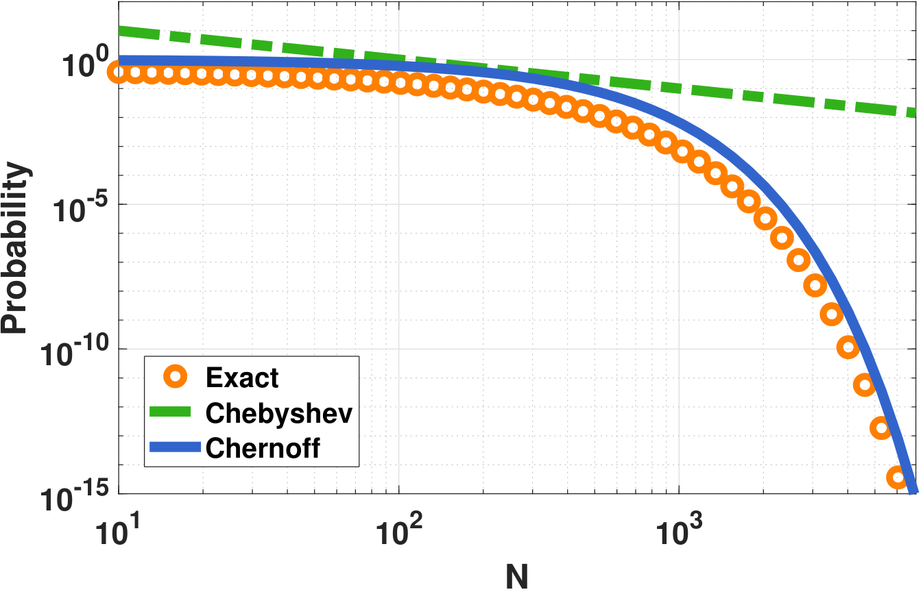
\begin{aligned} \Pb[ X \ge \varepsilon] &\le e^{-\varphi(\varepsilon)} = \exp\left\{-\frac{\varepsilon^2 N}{2\sigma^2}\right\}. \end{aligned}

■

Figure 6.9 shows the comparison between the exact probability, the bound provided by Chebyshev's inequality, and Chernoff's bound:

sep0ex
Exact: $\Pb[X \ge \varepsilon] = 1-\Phi\left(\frac{\sqrt{N}\varepsilon}{\sigma}\right)$.
Chebyshev: $\Pb[X \ge \varepsilon] \le \frac{\sigma^2}{N\varepsilon^2}$,
Chernoff: $\Pb\left[ X \ge \varepsilon \right] \le \exp\left\{-\frac{\varepsilon^2 N}{2\sigma^2}\right\}$.

In this numerical experiment, we set $\varepsilon = 0.1$, and $\sigma = 1$. We vary the number $N$. As we can see from the figure, the bound provided by Chebyshev is valid but very loose. It does not even capture the tail as $N$ grows. On the other hand, Chernoff's bound is reasonably tight. However, one should note that the tightness of Chernoff is only valid for large $N$. When $N$ is small, it is possible to construct random variables such that Chebyshev is tighter.

**Figure 6.9.** Comparison between Chernoff's bound and Chebyshev's bound. The random variable we use is $X \sim \text{Gaussian}(0,\sigma^2/N)$. As $N$ grows, we show the probability bounds predicted by the two methods.

The MATLAB code used to generate this plot is illustrated below.

MATLAB

% MATLAB code to compare the probability bounds
    epsilon = 0.1;
    sigma   = 1;
    N       = logspace(1,3.9,50);
    p_exact = 1-normcdf(sqrt(N)*epsilon/sigma);
    p_cheby = sigma^2./(epsilon^2*N);
    p_chern = exp(-epsilon^2*N/(2*sigma^2));
    
    loglog(N, p_exact, '-o', 'Color', [1 0.5 0], 'LineWidth', 2); hold on;
    loglog(N, p_cheby, '-', 'Color', [0.2 0.7 0.1], 'LineWidth', 2);
    loglog(N, p_chern, '-', 'Color', [0.2 0.0 0.8], 'LineWidth', 2);

What could go wrong if we insist on using Chebyshev's inequality? Consider the following example.

Example 6.9

Let $X \sim \text{Gaussian}(0,\sigma^2/N)$. Suppose that we want the probability to be no greater than a confidence level of $\alpha$:

\begin{aligned} \Pb[ X \ge \varepsilon] \le \alpha. \end{aligned}

Let $\alpha = 0.05$, $\varepsilon = 0.1$, and $\sigma = 1$. Find the $N$ using (i) Chebyshev's inequality and (ii) Chernoff's inequality.

Solution

: (i) Chebyshev's inequality implies that

\begin{aligned} \Pb[ X \ge \varepsilon] \le \frac{\sigma^2}{N\varepsilon^2} \le \alpha, \end{aligned}

which means that

N \ge \frac{\sigma^2}{\alpha \varepsilon^2}.

If we plug in $\alpha = 0.05$, $\varepsilon = 0.1$, and $\sigma = 1$, then $N \ge 2000$.

(ii) For Chernoff's inequality, it holds that

\begin{aligned} \Pb[ X \ge \varepsilon] \le \exp\left\{-\frac{\varepsilon^2 N}{2\sigma^2}\right\} \le \alpha, \end{aligned}

which means that

N \ge -\frac{2\sigma^2}{\varepsilon^2} \log \alpha

Plugging in $\alpha = 0.05$, $\varepsilon = 0.1$, and $\sigma = 1$, we have that $N \ge 600$. This is more than 3 times smaller than the one predicted by Chebyshev's inequality. Which one is correct? Both are correct but Chebyshev's inequality is overly conservative. If $N \ge 600$ can make $\Pb[ X \ge \varepsilon] \le \alpha$, then certainly $N \ge 2000$ will work too. However, $N \ge 2000$ is too loose.

6.2.8Hoeffding's inequality

Chernoff's bound can be used to derive many powerful inequalities. Here we present an inequality for bounded random variables. This result is known as Hoeffding's inequality.

Theorem 6.15 (Hoeffding's inequality)

Let $X_1,\ldots,X_N$ be i.i.d. random variables with $0 \le X_n \le 1$, and $\E[X_n ] = \mu$. Then

\Pb\bigg[ \left|\overline{X}_N - \mu \right| > \epsilon \bigg] \le 2 e^{-2\epsilon^2 N},

where $\overline{X}_N = \frac{1}{N} \sum_{n=1}^N X_n$.

You may skip the proof of Hoeffding's inequality if this is your first time reading the book.

Proof. (Hoeffding's inequality) First, we show that

\begin{aligned} \Pb\big[\overline{X}_N - \mu > \epsilon\big] &= \Pb\left[\frac{1}{N}\sum_{n=1}^N X_n - \mu > \epsilon \right] = \Pb\left[\sum_{n=1}^N (X_n - \mu) > N\epsilon \right] \\ &= \Pb\left[e^{s\sum_{n=1}^N (X_n - \mu)} \ge e^{s\epsilon N}\right] \\ &\le \frac{\E[e^{s\sum_{n=1}^N (X_n-\mu)}]}{e^{s \epsilon N}} = \left(\frac{\E[e^{s (X_n-\mu)}]}{e^{s \epsilon}}\right)^N. \end{aligned}

Let $Z_n = X_n - \mu$. Then $-\mu \le Z_n \le 1 - \mu$. At this point we use Hoeffding Lemma (see below) that $\E[e^{sZ_n}] \le e^{\frac{s^2}{8}}$ because $b-a = (1-\mu)-(-\mu) = 1$. Thus,

\begin{aligned} \Pb\big[\overline{X}_N - \mu > \epsilon\big] &\le \left(\frac{\E[e^{s Z_n}]}{e^{s \epsilon}}\right)^N \le \left( \frac{e^{\frac{s^2}{8}}}{e^{s\epsilon}}\right)^N = e^{\frac{s^2N}{8}-s\epsilon N}, \qquad \forall s. \end{aligned}

This result holds for all $s$, and thus it holds for the $s$ that minimizes the right-hand side. This implies that

\begin{aligned} \Pb\big[\overline{X}_N - \mu > \epsilon\big] &\le \min_s \left\{\exp\left\{\frac{s^2 N}{8}-s\epsilon N\right\}\right\}. \end{aligned}

Minimizing the exponent gives $\frac{d}{ds} \left\{\frac{s^2 N}{8} - s\epsilon N\right\} = \frac{sN}{4} - \epsilon N = 0$. Thus we have $s = 4\epsilon$. Hence,

\begin{aligned} \Pb\big[\overline{X}_N - \mu > \epsilon\big] &\le \exp\bigg\{ \frac{(4\epsilon)^2 N}{8} - (4\epsilon)\epsilon N\bigg\} = e^{-2\epsilon^2 N}. \end{aligned}

By symmetry, $\Pb\big[\overline{X}_N - \mu < -\epsilon\big] \le e^{-2\epsilon^2 N}$. Then by union bound we show that

\begin{aligned} \Pb\big[|\overline{X}_N - \mu| > \epsilon\big] &= \Pb\big[\overline{X}_N - \mu > \epsilon\big] + \Pb\big[\overline{X}_N - \mu < -\epsilon\big] \\ &\le e^{-2\epsilon^2 N} + e^{-2\epsilon^2 N} \\ &= 2e^{-2\epsilon^2 N}. \end{aligned}

■

Lemma 6.3 (Hoeffding's lemma)

Let $a \le X \le b$ be a random variable with $\E[X] = 0$. Then

M_X(s) \bydef \E\left[e^{s X}\right]\le \exp\left\{\frac{s^2(b-a)^2}{8}\right\}.

Proof. Since $a \le X \le b$, we can write $X$ as a linear combination of $a$ and $b$:

X = \lambda b + (1-\lambda)a,

where $\lambda = \frac{X-a}{b-a}$. Since $\exp(\cdot)$ is a convex function, it follows that $e^{\lambda b + (1-\lambda)a} \le \lambda e^b + (1-\lambda) e^a$. (Recall that $h$ is convex if $h(\lambda x + (1-\lambda)y) \le \lambda h(x) + (1-\lambda)h(y)$.) Therefore, we have

\begin{aligned} e^{sX} &\le \lambda e^{sb} + (1-\lambda) e^{sa} \\ &= \frac{X-a}{b-a}e^{sb} + \frac{b-X}{b-a}e^{sa}. \end{aligned}

Taking expectations on both sides of the equation,

\begin{aligned} \E[e^{sX}] &\le \frac{-a}{b-a}e^{sb} + \frac{b}{b-a}e^{sa}, \end{aligned}

because $\E[X] = 0$. Now, if we let $\theta = -\frac{a}{b-a}$, then

\begin{aligned} \frac{-a}{b-a}e^{sb} + \frac{b}{b-a}e^{sa} &= \theta e^{sb} + (1-\theta)e^{sa} \\ &= e^{sa} \left(1 - \theta + \theta e^{s(b-a)}\right) = \left(1 - \theta + \theta e^{s(b-a)}\right) e^{-s\theta(b-a)} \\ &= \left(1 - \theta + \theta e^{u}\right)e^{-\theta u} = e^{-\theta u + \log(1-\theta+\theta e^u)}, \end{aligned}

where we let $u = s(b-a)$. This can be simplified as $\E[e^{sX}] \le e^{\phi(u)}$ by defining

\phi(u) = -\theta u + \log(1-\theta+\theta e^u).

The final step is to approximate $\phi(u)$. To this end, we use Taylor approximation:

\begin{aligned} \phi(u) &= \phi(0) + u \phi'(0) + \frac{u^2}{2}\phi''(\xi), \end{aligned}

for some $\xi \in [a,b]$. Since $\phi(0) = 0$, $\phi'(0) = 0$, and $\phi''(u) \le \frac{1}{4}$ for all $u$, it follows that

\begin{aligned} \phi(u) &= \frac{u^2}{2}\phi''(\xi) \le \frac{u^2}{8} = \frac{s^2(b-a)^2}{8}. \end{aligned}

■

End of the proof.

What is so special about the Hoeffding's inequality?

sep0ex
Since Hoeffding's inequality is derived from Chernoff's bound, it inherits the tightness. Hoeffding's inequality is much stronger than Chebyshev's inequality in bounding the tail distributions.
Hoeffding's inequality is one of the few inequalities that do not require $\E[X]$ and $\Var[X]$ on the right-hand side.
A downside of the inequality is that boundedness is not always easy to satisfy. For example, if $X_n$ is a Gaussian random variable, Hoeffding does not apply. There are more advanced inequalities for situations like these.

Interpreting Hoeffding's inequality. One way to interpret Hoeffding's inequality is to write the equation as

\Pb\big[ \left|\overline{X}_N - \mu \right| > \epsilon \big] \le \underset{\delta}{\underbrace{2 e^{-2\epsilon^2 N}}},

which is equivalent to

\Pb\big[ \left|\overline{X}_N - \mu \right| \le \epsilon \big] \ge 1-\delta.

This means that with a probability at least $1-\delta$, we have

\overline{X}_N - \epsilon \le \mu \le \overline{X}_N + \epsilon.

If we let $\delta = 2e^{-2\epsilon^2 N}$, this becomes

\overline{X}_N - \sqrt{\frac{1}{2N}\log\frac{2}{\delta}} \le \mu \le \overline{X}_N + \sqrt{\frac{1}{2N}\log\frac{2}{\delta}}.

This inequality is a confidence interval (see Chapter 9). It says that with probability at least $1-\delta$, the interval $[\overline{X}_N-\epsilon, \; \overline{X}_N+\epsilon]$ includes the true population mean $\mu$.

There are two questions one can ask about the confidence interval:

sep0ex
Given $N$ and $\delta$, what is the confidence interval? Eq. (6.28) tells us that if we know $N$, to achieve a probability of at least $1-\delta$ the confidence interval will follow Eq. (6.28). For example, if $N =$ 10,000 and $\delta = 0.01$, $\sqrt{\frac{1}{2N}\log\frac{2}{\delta}} = 0.016$. Therefore, with a probability at least 99%, the true population mean $\mu$ will be included in the interval
$\overline{X}_N - 0.016 \le \mu \le \overline{X}_N + 0.016.$
If we want to achieve a certain confidence interval, what is the $N$ we need? If we are given $\epsilon$ and $\delta$, the $N$ we need is
$\delta \le 2e^{-2\epsilon^2 N} \quad \Rightarrow \quad N \ge \frac{\log \frac{2}{\delta}}{2\epsilon^2}.$
For example, if $\delta = 0.01$ and $\epsilon = 0.01$, the $N$ we need is $N \ge 26,500$.

When is Hoeffding's inequality used? Hoeffding's inequality is fundamental in modern machine learning theory. In this field, one often wants to quantify how well a learning algorithm performs with respect to the complexity of the model and the number of training samples. For example, if we choose a complex model, we should expect to use more training samples or overfit otherwise. Hoeffding's inequality provides an asymptotic description of the training error, testing error, and the number of training samples. The inequality is often used to compare the theoretical performance limit of one model versus another model. Therefore, although we do not need to use Hoeffding's inequality in this book, we hope you appreciate its tightness.

Closing Remark. We close this section by providing the historic context of Chernoff's inequality. Herman Chernoff, the discoverer of Chernoff's inequality, wrote the following many years after the publication of the original paper in 1952.

“In working on an artificial example, I discovered that I was using the Central Limit Theorem for large deviations where it did not apply. This led me to derive the asymptotic upper and lower bounds that were needed for the tail probabilities. [Herman] Rubin claimed he could get these bounds with much less work, and I challenged him. He produced a rather simple argument, using Markov's inequality, for the upper bound. Since that seemed to be a minor lemma in the ensuing paper I published (Chernoff, 1952), I neglected to give him credit. I now consider it a serious error in judgment, especially because his result is stronger for the upper bound than the asymptotic result I had derived.” — Herman Chernoff, “A career in statistics,” in Lin et al., Past, Present, and Future of Statistical Science (2014), p. 35.