Law of Large Numbers

In this section, we present our first main result: the law of large numbers. We will discuss two versions of the law: the weak law and the strong law. We will also introduce two forms of convergence: convergence in probability and almost sure convergence.

6.3.1Sample average

The law of large numbers is a probabilistic statement about the sample average. Suppose that we have a collection of i.i.d. random variables \(X_1,\ldots,X_N\). The sample average of these \(N\) random variables is defined as follows:

If the random variables \(X_1,\ldots,X_N\) are i.i.d. so that they have the same population mean \(\E[X_n] = \mu\) (for \(n = 1,\ldots,N\)), then by the linearity of the expectation,

Therefore, the mean of \(\overline{X}_N\) is the population mean \(\mu\).

The sample average, \(\overline{X}_N\), plays an important role in statistics. For example, by surveying 10,000 Americans, we can find a sample average of their ages. Since we never have access to the true population mean, the sample average is an estimate, and since \(\overline{X}_N\) is only an estimate, we need to ask how good the estimate is.

One reason we ask this question is that \(\overline{X}_N\) is a finite-sample “approximation” of \(\mu\). More importantly, the root of the problem is that \(\overline{X}_N\) itself is a random variable because \(X_1, \ldots, X_N\) are all random variables. Since \(\overline{X}_N\) is a random variable, there is a PDF of \(\overline{X}_N\); there is a CDF of \(\overline{X}_N\); there is \(\E[\overline{X}_N]\); and there is \(\Var[\overline{X}_N]\). Since \(\overline{X}_N\) is a random variable, it has uncertainty. To say that we are confident about \(\overline{X}_N\), we need to ensure that the uncertainty is within some tolerable range.

How do we control the uncertainty? We can compute the variance. If \(X_1,\ldots,X_N\) are i.i.d. random variables with the same variance \(\Var[X_n] = \sigma^2\) (for \(n = 1,\ldots, N\)), then

Therefore, the variance will shrink to 0 as \(N\) grows. In other words, the more samples we use to construct the sample average, the less deviation the random variable \(\overline{X}_N\) will have.

Visualizing the sample average

To help you visualize the randomness of \(\overline{X}_N\), we consider an experiment of drawing \(N\) Bernoulli random variables \(X_1,\ldots,X_N\) with parameter \(p = 1/2\). Since \(X_n\) is Bernoulli, it follows that

We construct a sample average \(\overline{X}_N = \frac{1}{N}\sum_{n=1}^N X_n\). Since \(X_n\) is a Bernoulli random variable, we know everything about \(\overline{X}_N\). First, \(\overline{X}_N\) is a binomial random variable, since \(\overline{X}_N\) is the sum of Bernoulli random variables. Second, the mean and variance of \(\overline{X}_N\) are respectively

In Figure 6.10, we plot the random variables \(\overline{X}_N\) (the black crosses) for every \(N\). You can see that at each \(N\), e.g., \(N = 100\), there are many possible observations for \(\overline{X}_N\) because \(\overline{X}_N\) itself is a random variable. As \(N\) increases, we see that the deviation of the random variables becomes smaller. In the same plot, we show the bounds \(\mu \pm 3\sigma_{\overline{X}_N}\), which are three standard deviations from the mean. We can see clearly that the bounds provide a very good envelope covering the random variables. As \(N\) goes to infinity, we can see that the standard deviation goes to zero, and so \(\overline{X}_N\) approaches the true mean.

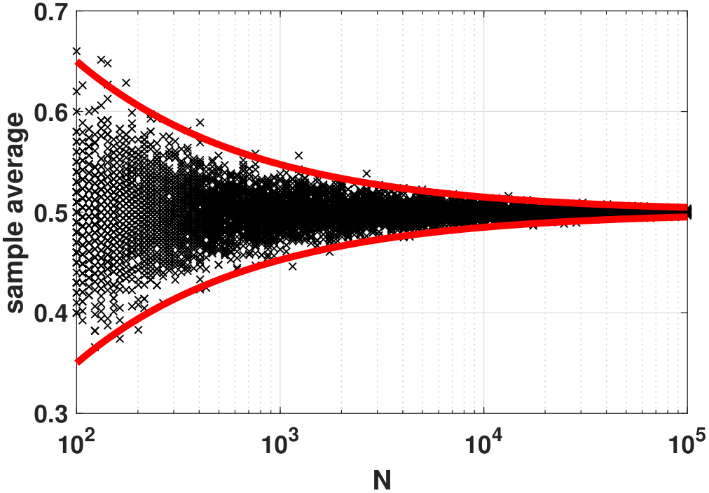
For your reference, the MATLAB code and the Python code we used to generate the plot are shown below.

% MATLAB code to illustrate the weak law of large numbers
    Nset = round(logspace(2,5,100));
    for i=1:length(Nset)
        N = Nset(i);
        p = 0.5;
        x(:,i) = binornd(N, p, 1000,1)/N;
    end
    y = x(1:10:end,:)';
    semilogx(Nset, y, 'kx'); hold on;
    semilogx(Nset, p+3*sqrt(p*(1-p)./Nset), 'r', 'LineWidth', 4);
    semilogx(Nset, p-3*sqrt(p*(1-p)./Nset), 'r', 'LineWidth', 4);

# Python code to illustrate the weak law of large numbers
    import numpy as np
    import matplotlib.pyplot as plt
    import scipy.stats as stats
    import numpy.matlib
    p = 0.5
    Nset = np.round(np.logspace(2,5,100)).astype(int)
    x = np.zeros((1000,Nset.size))
    for i in range(Nset.size):
      N = Nset[i]
      x[:,i] = stats.binom.rvs(N, p, size=1000)/N
    Nset_grid = np.matlib.repmat(Nset, 1000, 1)
    
    plt.semilogx(Nset_grid, x,'ko');
    plt.semilogx(Nset, p + 3*np.sqrt((p*(1-p))/Nset), 'r', linewidth=6)
    plt.semilogx(Nset, p - 3*np.sqrt((p*(1-p))/Nset), 'r', linewidth=6)

Note the outliers for each \(N\) in Figure 6.10. For example, at \(N = 10^2\) we see a point located near 0.7 on the \(y\)-axis. This point is outside three standard deviations. Is it normal? Yes. Being outside three standard deviations only says that the probability of having this outlier is small. It does not say that the outlier is impossible. Having a small probability does not exclude the possibility. By contrast, if you say that something will surely not happen you mean that there is not even a small probability. The former is a weaker statement than the latter. Therefore, even though we establish a three standard deviation envelope, there are points falling outside the envelope. As \(N\) grows, the chance of having a bad outlier becomes smaller. Therefore, the greater the \(N\), the smaller the chance we will get an outlier.

If the random variables \(X_n\) are i.i.d., the above phenomenon is universal. Below is an example of the Poisson case.

6.3.2Weak law of large numbers (WLLN)

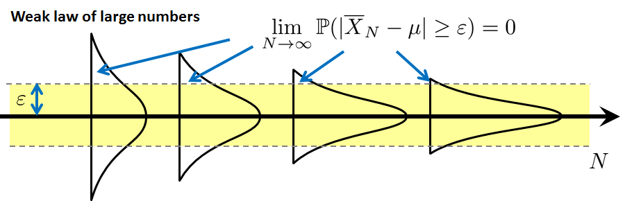
The analysis of Figure 6.10 shows us something important, namely that the convergence in a probabilistic way is different from that in a deterministic way. We now describe one fundamental result related to probabilistic convergence, known as the weak law of large numbers.

The weak law of large numbers is portrayed graphically in Figure 6.11. In this figure we draw several PDFs of the sample average \(\overline{X}_N\). The shapes of the PDFs are getting narrower as the variance of the random variable shrinks. Since the PDFs become narrower, the probability \(\Pb[|\overline{X}_N-\mu| > \varepsilon]\) becomes more unlikely. At the limit when \(N \rightarrow \infty\), the probability vanishes. The weak law of large numbers asserts that this happens for any set of i.i.d. random variables. It says that the sequence of probability values \(\delta_N \bydef \Pb[|\overline{X}_N-\mu| > \varepsilon]\) will converge to zero.

6.3.3Convergence in probability

The example above tells us that in order to show convergence, we need to first compute the probability \(\delta_n\) of each event and then take the limit of the sequence, e.g., the one shown in the table below:

Therefore, the convergence is the convergence of the probability. Since \(\{\delta_1,\delta_2,\ldots\}\) is a sequence of real numbers (between 0 and 1), any convergence results for real numbers apply here.

Note that the convergence controls only the probabilities. Probability means chance. Therefore, having the limit converging to zero only means that the chance of happening is becoming smaller and smaller. However, at any \(N\), there is still a chance that some bad event can happen.

What do we mean by a bad event? Assume that \(X_n\) are fair coins. The sample average \(\overline{X}_N = (1/N)\sum_{n=1}^N X_n\) is more or less equal to 1/2 as \(N\) grows. However, even if \(N\) is a large number, say \(N = 1000\), we are still not certain that the sample average is exactly 1/2. It is possible, though very unlikely, that we obtain \(1000\) heads or \(1000\) tails (so that the sample average is “1” or “0”). The bottom line is: Having a probability converging to zero only means that for any tolerance level we can always find an \(N\) large enough so that the probability is smaller than that tolerance.

The type of convergence described by the weak law of large numbers is known as the convergence in probability.

The following two examples illustrate how to prove convergence in probability.

Example 6.12

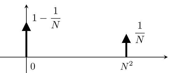
Construct an example such that \(A_N\) converges in probability to something, but \(\E[A_N]\) does not converge to the same thing.

Solution

Consider a sequence of random variables \(A_N\) such that

$$\Pb[A_N = \alpha] = \begin{cases} 1-\frac{1}{N}, &\qquad \alpha = 0,\\ \frac{1}{N}, &\qquad \alpha = N^2,\\ 0, &\qquad \text{otherwise}. \end{cases}$$

The PDF of the random variable \(A_N\) is shown in Figure 6.12.

We first show that \(A_N\) converges in probability to zero. Let \(\varepsilon> 0\) be a fixed constant. Since \(\varepsilon> 0\),

$$\Pb[A_N \ge \varepsilon] = \frac{1}{N}$$

for any \(N > \sqrt{\varepsilon}\). Therefore, we have that

$$\begin{aligned} \lim_{N \rightarrow \infty} \; \Pb[|A_N-0|\ge\varepsilon] &= \lim_{N\rightarrow \infty} \Pb[A_N \ge \varepsilon]\\ &= \lim_{N\rightarrow \infty} \frac{1}{N} = 0. \end{aligned}$$

Hence, \(A_N\) converges to 0 in probability.

However, \(\E[A_N]\) does not converge to zero, because

$$\begin{aligned} \E[A_N] &= 0\cdot \left(1-\frac{1}{N}\right) + N^2 \cdot \frac{1}{N} \\ &= N. \end{aligned}$$

So \(\E[A_N]\) goes to infinity as \(N\) grows.

6.3.4Can we prove WLLN using Chernoff's bound?

In proving WLLN we use Chebyshev's inequality. Can we use Chernoff's inequality (or Hoeffding's) to prove the result? Yes, we can use them. However, notice that the task here is to prove convergence, not to find the best convergence. Finding the best convergence means finding the fastest decay rate of the probability sequence. Chernoff's bound (and Hoeffding's inequality) offers a better decay rate. However, Chernoff's bound needs to be customized for individual random variables. For example, Chernoff's bound for Gaussian is different from Chernoff's bound for exponential. This result makes Chebyshev the most convenient bound because it only requires the variance to be bounded.

What if we insist on using Chernoff's bound in proving the WLLN? We can do that for specific random variables. Let's consider two examples. The first example is the Gaussian random variable where \(X_n \sim \calN(0,\sigma^2)\). We know that \(\overline{X}_N \sim \calN(0, \sigma^2/N)\). Chernoff's bound shows that

Taking the limit on both sides, we have

Note that the rate of convergence here is exponential. The rate of convergence offered by Chebyshev is only linear. Of course, you may argue that since \(X_n\) is Gaussian we have closed-form expressions about the probability, so we do not need Chernoff's bound. This is a legitimate point, and so here is an example where we do not have a closed-form expression for the probability.

Consider a sequence of arbitrary i.i.d. random variables \(X_1,\ldots,X_N\) with \(0 \le X_n \le 1\). Then Hoeffding's inequality tells us that

Taking the limit on both sides, we have

Again, we obtain a WLLN result, this time for i.i.d. random variables \(X_1,\ldots,X_N\) with \(0 \le X_n \le 1\).

As you can see from these two examples, WLLN can be proved in multiple ways depending on how general the random variables need to be.

6.3.5Does the weak law of large numbers always hold?

The weak law of large numbers does not always hold. Recall that when we prove the weak law of large numbers using Chebyshev's inequality, we implicitly require that the variance \(\Var[\overline{X}_N]\) is finite. (Look at the condition that \(\E[X^2] < \infty\).) Thus for distributions whose variance is unbounded, Chebyshev's inequality does not hold. One example is the Cauchy distribution. The PDF of a Cauchy distribution is

where \(\gamma\) is a parameter. Letting \(\gamma = 1\),

Since the second moment is unbounded, the variance of \(X\) will also be unbounded.

A perceptive reader may observe that even if \(\E[X^2]\) is unbounded, it does not mean that the tail probability is unbounded. This is correct. However, for Cauchy distributions, we can show that the sample average \(\overline{X}_N\) does not converge to the mean when \(N \rightarrow \infty\) (and so the WLLN fails). To see this, we note that

So for the sample average \(\overline{X}_N = \frac{1}{N}\sum_{n=1}^N X_n\), the characteristic function is

which remains a Cauchy distribution with \(\gamma = 1\). Therefore, we have that

Thus no matter how many samples we have, \(\Pb[|\overline{X}_N| \le \varepsilon]\) will never converge to 1 (so \(\Pb[|\overline{X}_N| > \varepsilon]\) will never converge to 0). Therefore, WLLN does not hold.

6.3.6Strong law of large numbers

Since there is a “weak” law of large numbers, you will not be surprised to learn that there is a strong law of large numbers. The strong law is more restrictive than the weak law. Any sequence satisfying the strong law will satisfy the weak law, but not vice versa. Since the strong law is “stronger”, the proof is more involved.

The strong law flips the order of limit and probability. As you can see, the difference between the strong law and the weak law is the order of the limit and the probability. In the weak law, the limit is outside the probability, whereas, in the strong law, the limit is inside the probability. This switch in order makes the interpretation of the result fundamentally different. In the final analysis, the weak law concerns the limit of a sequence of probabilities (which are just real numbers between 0 and 1). However, the strong law concerns the limit of a sequence of random variables. The strong law answers the question, what is the limiting object of the sample average as \(N\) grows?

The strong law concerns the limiting object, not a sequence of numbers. What is the “limiting object”? If we denote \(\overline{X}_N\) as the sample average using \(N\) samples, then we know that \(\overline{X}_1\) is a random variable, \(\overline{X}_2\) is a random variable, and all \(\overline{X}_n\)'s are random variables. So we have a sequence of random variables. As \(N\) goes to infinity, we can ask about the limiting object \(\lim_{N\rightarrow \infty}\overline{X}_N\). However, even without any deep analysis, you should be able to see that \(\lim_{N\rightarrow \infty}\overline{X}_N\) is another random variable. The strong law says that this limiting object will “successfully” become a deterministic number \(\mu\), after a finite number of “failures”.

The strong law asserts that there are a finite number of failures. Let us explain “success” and “failure”. \(\overline{X}_N\) is a random variable, so it fluctuates. However, as \(N\) goes to infinity, the strong law says that the number of times where \(\overline{X}_N \not= \mu\) will be zero. That is, there is a finite number of times where \(\overline{X}_N \not= \mu\) (i.e., fail), and afterward, you will be perfectly fine (i.e., success). Yes, perfectly fine means 100%. The weak law only guarantees 99.99%.

A good example for differentiating the weak law and the strong law is an electronic dictionary that improves itself every time you use it. The weak law says that if you use the dictionary for a long period, the probability of making an error will become small. You will still get an error once in a while, but the probability is very small. This is a 99.99% guarantee, and it is the weak law. The strong law says that the number of failures is finite. After you have gone through this finite number of failures, you will be completely free of error. This is a 100% guarantee by the strong law. When will you hit this magical number? The strong law does not say when; it only asserts the existence of this number. However, this existence is already good enough in many ways. It gives a certificate of assurance, whereas the weak law still has uncertainty.

Strong law \(\not=\) deterministic. If the strong law offers a 100% guarantee, does it mean that it is a deterministic guarantee? No, the strong law is still a probabilistic statement because we are still using \(\Pb[\cdot]\) to measure an event. The event can include measure-zero subsets, and the measure-zero subsets can be huge. For example, the set of rational numbers on the real line is a measure-zero set when measuring the probability using an integration. The strong law does not handle those measure-zero subsets.

6.3.7Almost sure convergence

The type of convergence used by the strong law of large numbers is the almost sure convergence. It is defined formally as follows.

To prove almost sure convergence, one needs to show that the sequence \(A_N\) will demonstrate \(A_N \not= \alpha\) for a finite number of times. Afterward, \(A_N\) needs to demonstrate \(A_N = \alpha\).

6.3.8Proof of the strong law of large numbers

The strong law of large numbers can be proved in several ways. We present a proof based on Bertsekas and Tsitsiklis, Introduction to Probability, Problems 5.16 and 5.17, which require a finite fourth moment \(\E[X_n^4] < \infty\). An alternative proof that requires only \(\E[X_n] < \infty\) is from Billingsley, Probability and Measure, Theorem 22.1.