eBook › Chapter 6 · Sample Statistics

Section 6.4

Central Limit Theorem

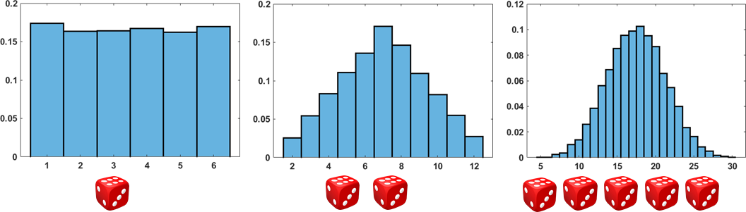
The law of large numbers tells us the mean of the sample average $\overline{X}_N = (1/N)\sum_{n=1}^N X_n$. However, if you recall our experiment of throwing $N$ dice and inspecting the PDF of the sum of the numbers, you may remember that the convolution of an infinite number of uniform distributions gives us a Gaussian distribution. For example, we show a sequence of experiments in Figure 6.13. In each experiment, we throw $N$ dice and count the sum. Therefore, if each face of the die is denoted as $X_n$, then the sum is $X_1 + \cdots + X_N$. We plot the PDF of the sum. As you can see in the figure, $X_1 + \cdots + X_N$ converges to a Gaussian. This phenomenon is explained by the Central Limit Theorem (CLT).

**Figure 6.13.** Pictorial illustration of the Central Limit Theorem. Suppose we throw a die and record the face. [Left] If we only have one die, then the distribution of the face is uniform. [Middle] If we throw two dice, the distribution is the convolution of two uniform distributions. This will give us a triangle distribution. [Right] If we throw five dice, the distribution is becoming similar to a Gaussian. The Central Limit Theorem says that as $N$ goes to infinity, the distribution of the sum will converge to a Gaussian.

What does the Central Limit Theorem say? Let $\overline{X}_N$ be the sample average, and let $Z_N = \sqrt{N}\left(\frac{\overline{X}_N-\mu}{\sigma}\right)$ be the normalized variable. The Central Limit Theorem is as follows:

The CDF of $Z_N$ is converging pointwise to the CDF of Gaussian(0,1).

Note that we are very careful here. We are not saying that the PDF of $Z_N$ is converging to the PDF of a Gaussian, nor are we saying that the random variable $Z_N$ is converging to a Gaussian random variable. We are only saying that the values of the CDF are converging pointwise. The difference is subtle but important.

To understand the difficulty and the core ideas, we first present the concept of convergence in distribution.

6.4.1Convergence in distribution

Definition 6.8

Let $Z_1,\ldots,Z_N$ be random variables with CDFs $F_{Z_1},\ldots,F_{Z_N}$ respectively. We say that a sequence of $Z_1,\ldots,Z_N$ converges in distribution to a random variable $Z$ with CDF $F_Z$ if

\lim_{N \rightarrow \infty}F_{Z_N}(z) = F_Z(z),

for every continuous point $z$ of $F_Z$. We write $Z_N \overset{d}{\rightarrow} Z$ to denote convergence in distribution.

This definition involves many concepts, which we will discuss one by one. However, the definition can be summarized in a nutshell as follows.

Convergence in distribution = values of the CDF converge.

Example 6.15

(Bernoulli) Consider flipping a fair coin $N$ times. Denote each coin flip as a Bernoulli random variable $X_n \sim \text{Bernoulli}(p)$, where $n = 1,2,\ldots,N$. Define $Z_N$ as the sum of $N$ Bernoulli random variables, so that

Z_N = \sum_{n=1}^N X_n.

We know that the resulting random variable $Z_N$ is a binomial random variable with mean $Np$ and variance $Np(1-p)$. Let us plot the PDF $f_{Z_N}(z)$ as shown in Figure 6.14.

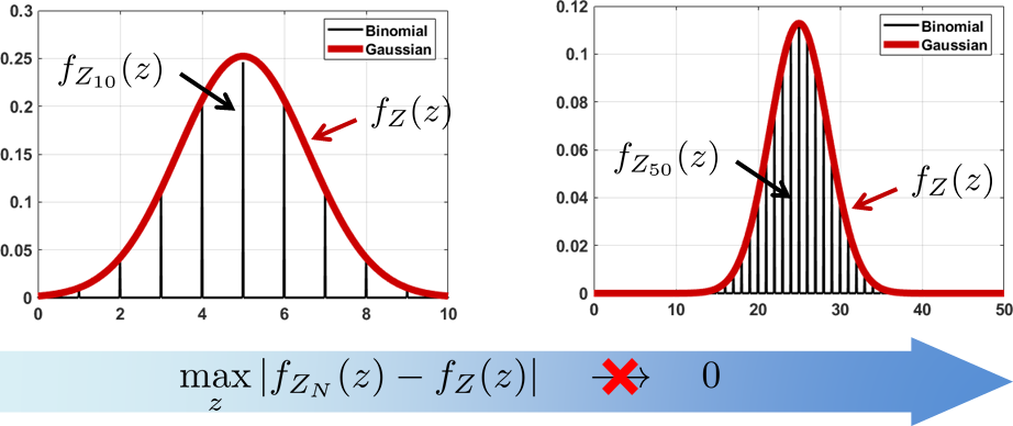
**Figure 6.14.** Convergence in distribution. The convergence in distribution concerns the convergence of the values of the CDF (not the PDF). In this figure, we let $Z_N = X_1+\cdots+X_N$, where $X_N$ is a Bernoulli random variable with parameter $p$. Since a sum of Bernoulli random variables is a binomial, $Z_N$ is a binomial random variable with parameters $(N,p)$. We plot the PDF of $Z_N$, which is a train of delta functions, and compare it with the Gaussian PDF. Observe that the error, $\max_z |f_{Z_N}(z) - f_Z(z)|$, does *not* converge to 0. The PDF of $Z_N$ is a binomial. A binomial is always a binomial. It will not turn into a Gaussian.

The first thing we notice in the figure is that as $N$ increases, the PDF of the binomial has an envelope that is “very Gaussian”. So one temptation is to say that the random variable $Z_N$ is converging to another random variable $Z$. In addition, we would think that the PDFs converge in the sense that for all $z$,

f_{Z_N}(z) = {N \choose z}p^{z}(1-p)^{N-z} \;\; \longrightarrow \;\; f_Z(z) = \frac{1}{\sqrt{2\pi\sigma^2}}\exp\left\{-\frac{(z-\mu)^2}{2\sigma^2}\right\},

where $\mu = Np$ and $\sigma^2 = Np(1-p)$.

Unfortunately this argument does not work, because $f_Z(z)$ is continuous but $f_{Z_N}(z)$ is discrete. The sample space of $Z_N$ and the sample space of $Z$ are completely different. In fact, if we write $f_{Z_N}$ as an impulse train, we observe that

f_{Z_N}(z) = \sum_{i=0}^N {N \choose i}p^{i}(1-p)^{N-i} \delta(z-i).

Clearly, no matter how big the $N$ is, the difference $|f_{Z_N}(z) - f_Z(z)|$ will never go to zero for non-integer values of $z$. Mathematically, we can show that

\max_{z} \; |f_{Z_N}(z) - f_Z(z)| \not\longrightarrow 0,

as $N \rightarrow \infty$. $Z_N$ is a binomial random variable regardless of $N$. It will not become a Gaussian.

If $f_{Z_N}(z)$ is not converging to a Gaussian PDF, how do we explain the convergence? The answer is to look at the CDF. For discrete PDFs such as a binomial random variable, the CDF is a staircase function. What we can show is that

F_{Z_N}(z) = \sum_{i=0}^{z} {N \choose i}p^{i}(1-p)^{N-i} \;\; \longrightarrow \;\; F_Z(z) = \int_{-\infty}^{z} \frac{1}{\sqrt{2\pi\sigma^2}}\exp\left\{-\frac{(t-\mu)^2}{2\sigma^2}\right\} \;dt.

The difference between the PDF convergence and the CDF convergence is that the PDF does not allow a meaningful “distance” between a discrete function and continuous function. For CDF, the distance is well defined by taking the difference between the staircase function and the continuous function. For example, we can compute

|F_{Z_N}(z) - F_Z(z)|, \qquad \text{for all continuous points $z$ of $F_Z$},

and show that

\max_z |F_{Z_N}(z) - F_Z(z)| \longrightarrow 0.

**Figure 6.15.** Convergence in distribution. This is the same as Figure 6.14, but this time we plot the CDF of $Z_N$. The CDF is a staircase function. We compare it with the Gaussian CDF. Observe that the error, $\max_z |F_{Z_N}(z) - F_Z(z)|$, converges to zero as $N$ grows. Convergence in distribution says that the sequence of CDFs $F_{Z_N}(z)$ will converge to the limiting CDF $F_Z(z)$, at all continuous points of $F_Z(z)$.

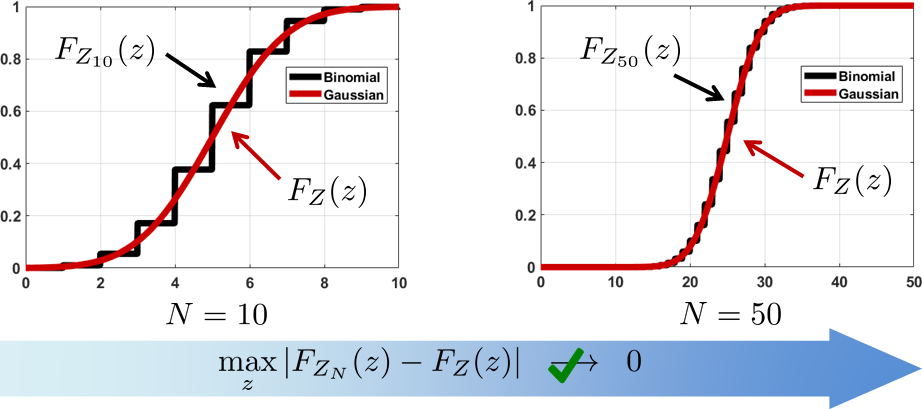
We need to pay attention to the set of $z$'s. We do not evaluate all $z$'s but only the $z$'s that are continuous points of $F_Z$. If $F_Z$ is Gaussian, this does not matter because all $z$'s are continuous. However, for CDFs containing discontinuous points, our definition of convergence in distribution will ignore these discontinuous points because they have a measure zero.

Example 6.16

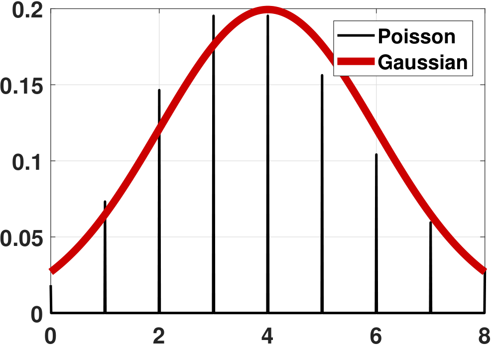
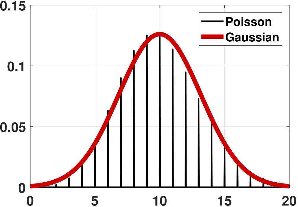
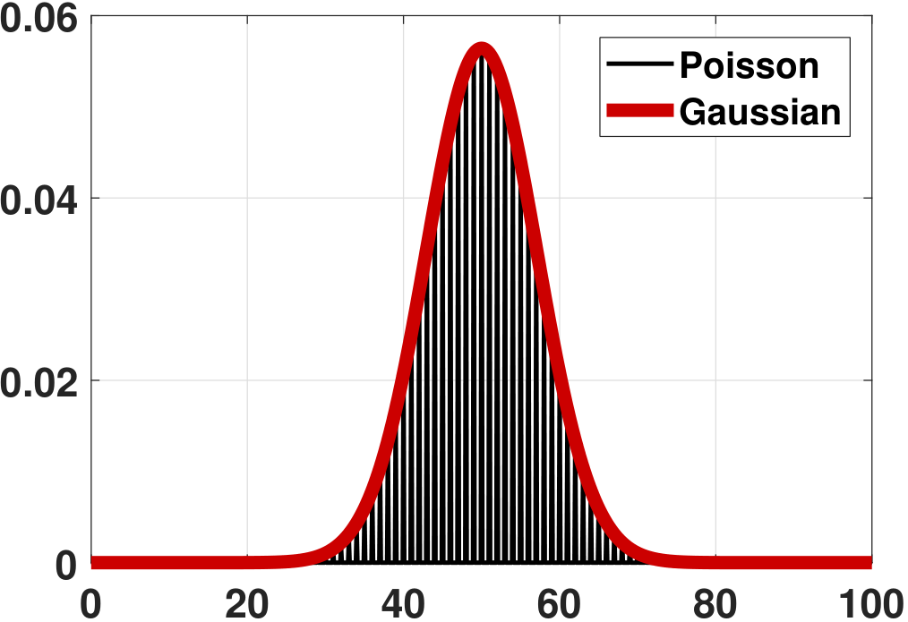
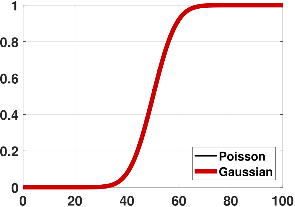
(Poisson) Consider $X_n \sim \text{Poisson}(\lambda)$, and consider $X_1,\ldots,X_N$. Define $Z_N = \sum_{n=1}^N X_n$. It follows that $\E[Z_N] = \sum_{n=1}^N \E[X_n] = N\lambda$ and $\Var[Z_N] = \sum_{n=1}^N \Var[X_n] = N\lambda$. Moreover, we know that the sum of Poissons remains a Poisson. Therefore, the PDF of $Z_N$ is

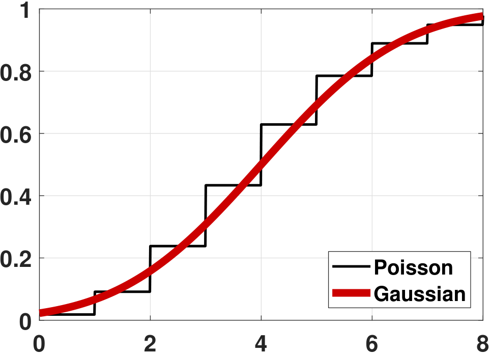
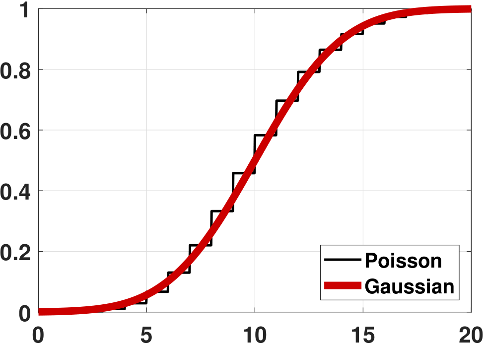
f_{Z_N}(z) = \sum_{k=0}^\infty \frac{(N\lambda)^k}{k!}e^{-N\lambda}\delta(z-k) \qquad\mbox{and}\qquad f_Z(z) = \frac{1}{\sqrt{2\pi\sigma^2}}\exp\left\{-\frac{(z-\mu)^2}{2\sigma^2}\right\},

where $\mu = N\lambda$ and $\sigma^2 = N\lambda$. Again, $f_{Z_N}$ does not converge to $f_Z$. However, if we compare the CDF, we can see from Figure 6.16 that the CDF of the Poisson is becoming better approximated by the Gaussian.

**Figure 6.16.** Convergence in distribution for a sum of Poisson random variables. Here we assume that $X_1,\ldots,X_N$ are i.i.d. Poisson with a parameter $\lambda$. We let $Z_N = \sum_{n=1}^N X_n$ be the sum, and compute the corresponding PDF (top row) and CDFs (bottom row). Just as with the binomial example, the PDFs of the Poisson do not converge but the CDFs of the Poisson converge to the CDF of a Gaussian.

Interpreting “convergence in distribution”. After seeing two examples, you should now have some idea of what “convergence in distribution” means. This concept applies to the CDFs. When we write

\lim_{N \rightarrow \infty}F_{Z_N}(z) = F_Z(z),

we mean that $F_{Z_N}(z)$ is converging to the value $F_Z(z)$, and this relationship holds for all the continuous $z$'s of $F_Z$. It does not say that the random variable $Z_N$ is becoming another random variable $Z$.

$Z_N \overset{d}{\longrightarrow} Z$ is equivalent to $\lim_{N \rightarrow \infty}F_{Z_N}(z) = F_Z(z)$.

Example 6.17

(Exponential) So far, we have studied the sum of discrete random variables. Now, let's take a look at continuous random variables. Consider $X_n \sim \text{Exponential}(\lambda)$, and let $X_1,\ldots,X_N$ be i.i.d. copies. Define $Z_N = \sum_{n=1}^N X_n$. Then $\E[Z_N] = \sum_{n=1}^N \E[X_n] = N/\lambda$ and $\Var[Z_N] = \frac{N}{\lambda^2}$. How about the PDF of $Z_N$? Using the characteristic functions, we know that

\begin{aligned} f_{X_n}(x) = \lambda e^{-\lambda x} \;\; \overset{\calF}{\longleftrightarrow} \;\; \Phi_{X_n}(j\omega) = \frac{\lambda}{\lambda+j\omega}. \end{aligned}

Therefore, the product is

\begin{aligned} \Phi_{Z_N}(j\omega) &= \prod_{n=1}^N \Phi_{X_n}(j\omega)= \frac{\lambda^N}{(\lambda+j\omega)^N} = \frac{\lambda^N}{(\lambda+j\omega)^N} \times \frac{(N-1)!}{(N-1)!}\\ &= \frac{\lambda^N}{(N-1)!} \cdot \frac{(N-1)!}{(\lambda+j\omega)^N} \overset{\calF}{\longleftrightarrow} \frac{\lambda^N}{(N-1)!}z^{N-1}e^{-\lambda z} = f_{Z_N}(z). \end{aligned}

This resulting PDF $f_{Z_N}(z) = \frac{\lambda^N}{(N-1)!}z^{N-1}e^{-\lambda z}$ is known as the Erlang distribution. The CDF of the Erlang distribution is

\begin{aligned} F_{Z_N}(z) &= \int_{-\infty}^z f_{Z_N}(t) \;dt \\ &= \int_{0}^z \frac{\lambda^N}{(N-1)!}t^{N-1}e^{-\lambda t} \;dt \\ &= \text{Gamma function}(z, N), \end{aligned}

where the last integral is known as the incomplete gamma function, evaluated at $z$.

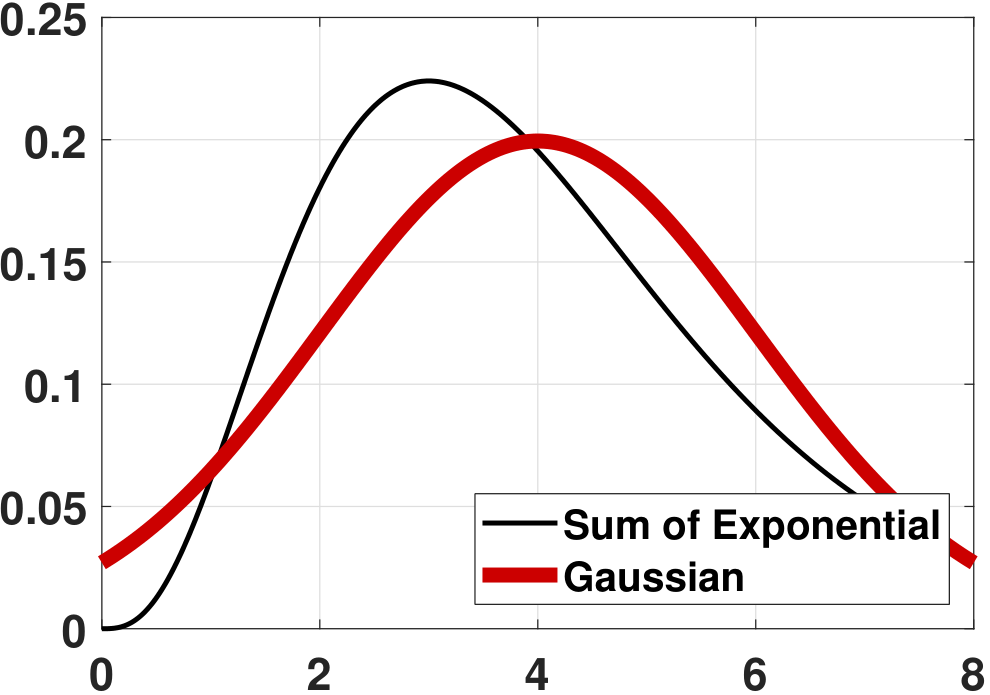
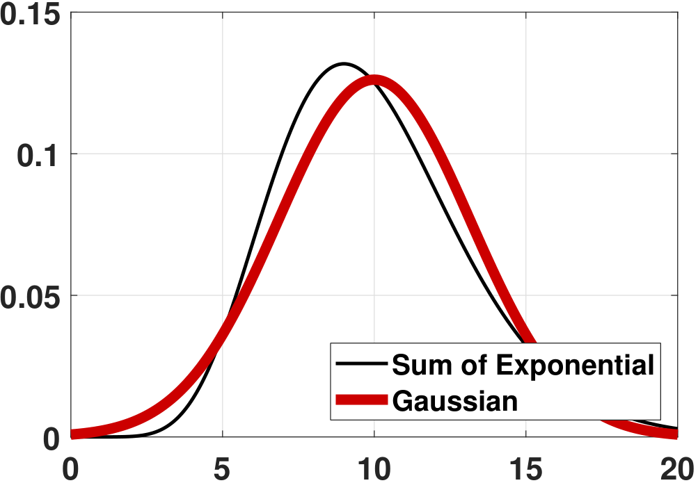
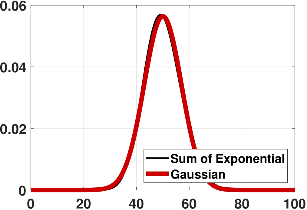
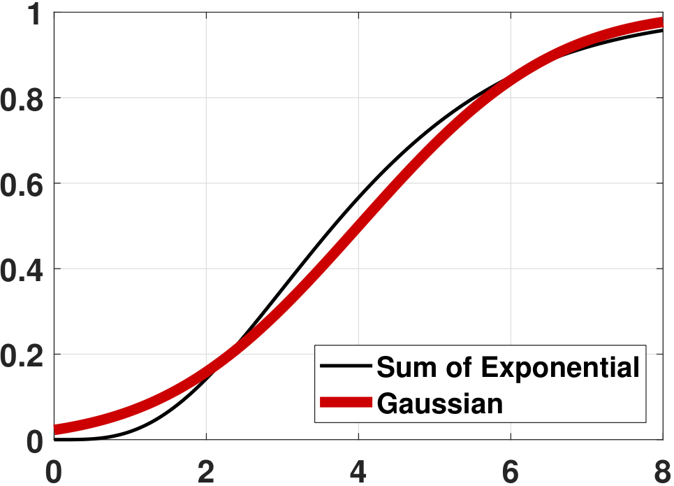
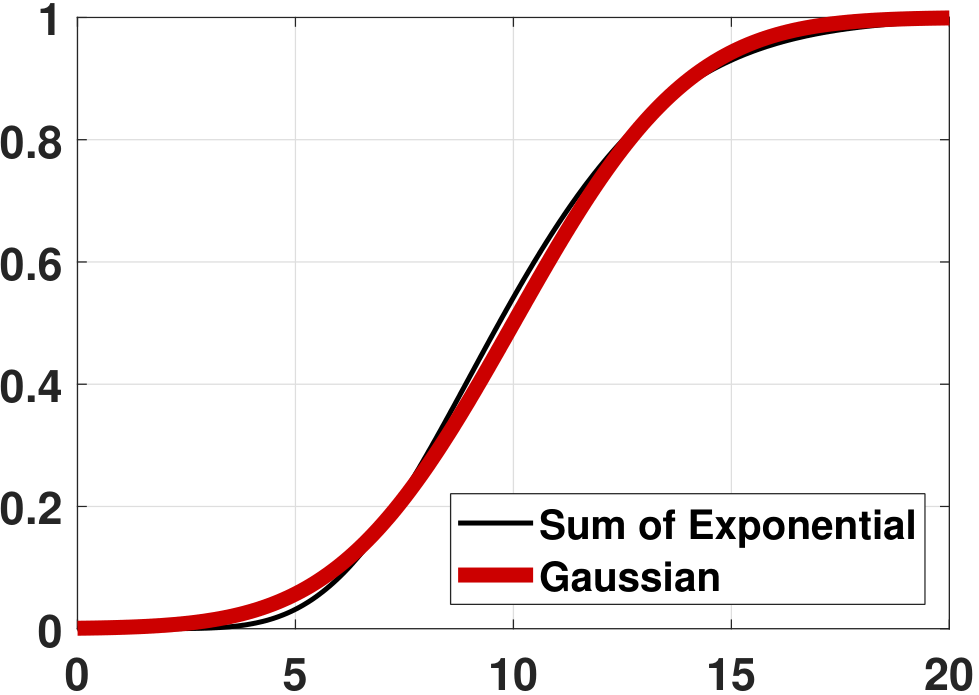
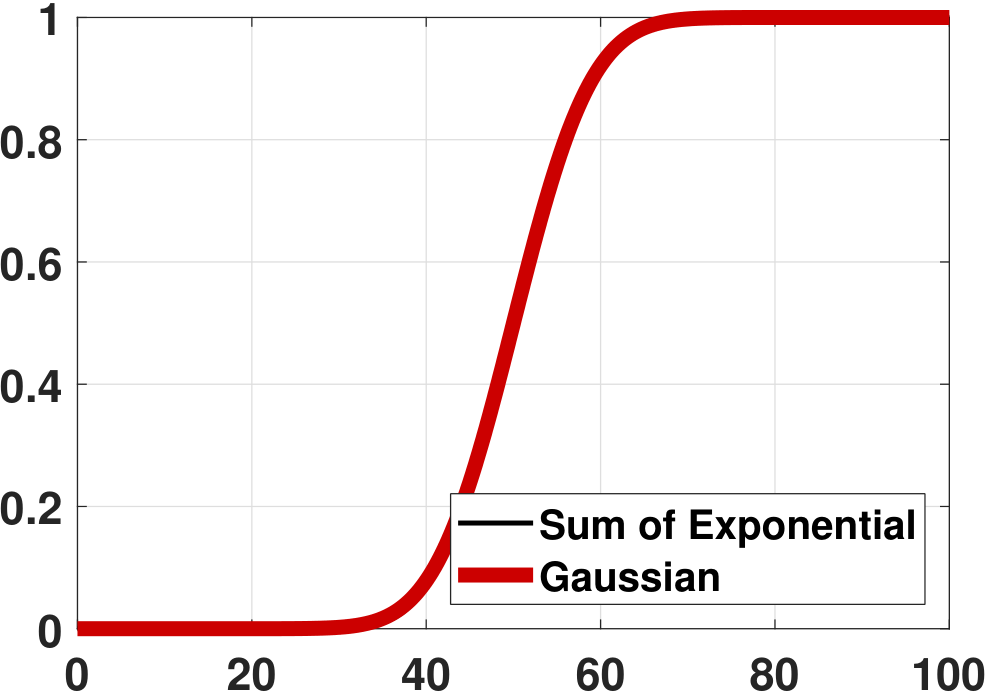
Given all of these, we can now compare the PDF and the CDF of $Z_N$ versus $Z$. Figure 6.17 shows the PDFs and the CDFs of $Z_N$ for various $N$ values. In this experiment we set $\lambda = 1$. As we can see from the experiment, the Erlang distribution's PDF and CDF converge to a Gaussian. In fact, for continuous random variables such as exponential random variables, we indeed have the random variable $Z_N$ converging to the random variable $Z$. This is quite different from discrete random variables, where $Z_N$ does not converge to $Z$ but only $F_{Z_N}$ converges to $F_Z$.

**Figure 6.17.** Convergence in distribution for a sum of exponential random variables. Here we assume that $X_1,\ldots,X_N$ are i.i.d. exponentials with a parameter $\lambda$. We define $Z_N = \sum_{n=1}^N X_n$ to be the sum. It is known that the sum of exponentials is an Erlang. We compute the corresponding PDF (top row) and CDFs (bottom row). Unlike the previous two examples, in this example we see that both PDFs and CDFs of the Erlang distribution are converging to a Gaussian.

Is $\overset{d}{\longrightarrow}$ stronger than $\overset{p}{\longrightarrow}$? Convergence in distribution is actually weaker than convergence in probability. Consider a continuous random variable $X$ with a symmetric PDF $f_X(x)$ such that $f_X(x) = f_X(-x)$. It holds that the PDF of $-X$ has the same PDF. If we define the sequence $Z_N = X$ if $N$ is odd and $Z_N = -X$ if $N$ is even, and let $Z = X$, then $F_{Z_N}(z) = F_Z(z)$ for every $z$ because the PDFs of $X$ and $-X$ are identical. Therefore, $Z_N \overset{d}{\rightarrow} Z$. However, $Z_N \not \overset{p}{\rightarrow} Z$ because $Z_N$ oscillates between the random variables $X$ and $-X$. These two random variables are different (although they have the same CDF) because $\Pb[X=-X] = \Pb[\{\omega: X(\omega)=-X(\omega)\}] = \Pb[\{\omega: X(\omega)=0\}] = 0$.

6.4.2Central Limit Theorem

Theorem 6.19 (Central Limit Theorem)

Let $X_1,\ldots,X_N$ be i.i.d. random variables of mean $\E[X_n] = \mu$ and variance $\Var[X_n] = \sigma^2$. Also, assume that $\E[|X_n^3|] < \infty$. Let $\overline{X}_N = (1/N) \sum_{n=1}^N X_n$ be the sample average, and let $Z_N = \sqrt{N}\left(\frac{\overline{X}_N-\mu}{\sigma}\right)$. Then

\lim_{N\rightarrow \infty} F_{Z_N}(z) = F_Z(z),

where $Z = \text{Gaussian}(0,1)$.

In plain words, the Central Limit Theorem says that the sample average (which is a random variable) has a CDF converging to the CDF of a Gaussian. Therefore, if we want to evaluate probabilities associated with the sample average, we can approximate the probability by the probability of a Gaussian.

As we discussed above, the Central Limit Theorem does not mean that the random variable $Z_N$ is converging to a Gaussian random variable, nor does it mean that the PDF of $Z_N$ is converging to the PDF of a Gaussian. It only means that the CDF of $Z_N$ is converging to the CDF of a Gaussian. Many people think that the Central Limit Theorem means “sample average converges to Gaussian”. This is incorrect for the above reasons. However, it is not completely wrong. For continuous random variables where both PDF and CDF are continuous, we will not run into situations where the PDF is a train of delta functions. In this case, convergence in CDF can be translated to convergence in PDF.

The power of the Central Limit Theorem is that the result holds for any distribution of $X_1,\ldots,X_N$. That is, regardless of the distribution of $X_1,\ldots,X_N$, the CDF of $\overline{X}_N$ is approaching a Gaussian.

Summary of the Central Limit Theorem

sep0ex
$X_1,\ldots,X_N$ are i.i.d. random variables, with mean $\mu$ and variance $\sigma^2$. They are not necessarily Gaussians.
Define the sample average as $\overline{X}_N = (1/N)\sum_{n=1}^N X_n$, and let $Z_N = \sqrt{N}\left(\frac{\overline{X}_N-\mu}{\sigma}\right)$.
The Central Limit Theorem says $Z_N \overset{d}{\longrightarrow} \text{Gaussian}(0,1)$. Equivalently, the theorem says that $\sqrt{N}(\overline{X}_N - \mu) \overset{d}{\longrightarrow} \text{Gaussian}(0,\sigma^2)$.
So if we want to evaluate the probability of $\overline{X}_N \in \calA$ for some set $\calA$, we can approximate the probability by evaluating the Gaussian:
$\Pb[ \overline{X}_N \in \calA] \approx \int_{\calA} \frac{1}{\sqrt{2\pi(\sigma^2/N)}} \exp\left\{-\frac{(y-\mu)^2}{2(\sigma^2/N)}\right\} \;dy.$
CLT does not say that the PDF of $\overline{X}_N$ is becoming a Gaussian PDF.
CLT only says that the CDF of $\overline{X}_N$ is becoming a Gaussian CDF.

If the set $\calA$ is an interval, we can use the standard Gaussian CDF to compute the probability.

Corollary 6.3

Let $X_1,\ldots,X_N$ be i.i.d. random variables with mean $\mu$ and variance $\sigma^2$. Define the sample average as $\overline{X}_N = (1/N)\sum_{n=1}^N X_n$. Then

\Pb[a \le \overline{X}_N \le b] \approx \Phi\left(\sqrt{N}\frac{b-\mu}{\sigma}\right) - \Phi\left(\sqrt{N}\frac{a-\mu}{\sigma}\right),

where $\Phi(z) = \int_{-\infty}^z \frac{1}{\sqrt{2\pi}}e^{-\frac{x^2}{2}}\;dx$ is the CDF of the standard Gaussian.

Proof. By the Central Limit Theorem, we know that $\overline{X}_N \overset{d}{\longrightarrow} \text{Gaussian}(\mu, \frac{\sigma^2}{N})$. Therefore,

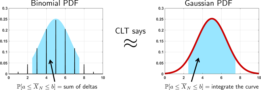
\begin{aligned} \Pb[a \le \overline{X}_N \le b] &\approx \int_{a}^{b} \frac{1}{\sqrt{2\pi(\sigma^2/N)}} \exp\left\{-\frac{(y-\mu)^2}{2(\sigma^2/N)}\right\} \;dy\\ &= \int_{\sqrt{N}\frac{a-\mu}{\sigma}}^{\sqrt{N}\frac{b-\mu}{\sigma}} \frac{1}{\sqrt{2\pi}}e^{-\frac{y^2}{2}}\;dy = \Phi\left(\sqrt{N}\frac{b-\mu}{\sigma}\right) - \Phi\left(\sqrt{N}\frac{a-\mu}{\sigma}\right). \end{aligned}

■

A graphical illustration of the CLT is shown in Figure 6.18, where we use a binomial random variable (which is the sum of i.i.d. Bernoulli) as an example. The CLT does not say that the binomial random variable is becoming a Gaussian. It only says that the probability covered by the binomial can be approximated by the Gaussian.

The following proof of the Central Limit Theorem can be skipped if this is your first time reading the book.

Proof of the Central Limit Theorem. We now give a “proof” of the Central Limit Theorem. Technically speaking, this proof does not prove the convergence of the CDF as the theorem claims; it only proves that the moment-generating function converges. The actual proof of the CDF convergence is based on the Berry-Esseen Theorem, which is beyond the scope of this book. However, what we prove below is still useful because it gives us some intuition about why Gaussian is the limiting random variable we should consider in the first place.

Let $Z_N = \sqrt{N}\left( \frac{\overline{X}_N - \mu}{\sigma}\right)$. It follows that $\E[Z_N] = 0$ and $\Var[Z_N] = 1$. Therefore, if we can show that $Z_N$ is converging to a standard Gaussian random variable $Z \sim \text{Gaussian}(0,1)$, then by the linear transformation property of Gaussian, $Y = \frac{\sigma}{\sqrt{N}} Z + \mu$ will be $\text{Gaussian}(\mu,\sigma^2/N)$.

Our proof is based on analyzing the moment-generating function of $Z_N$. In particular,

\begin{aligned} M_{Z_N}(s) \bydef \E[e^{sZ_N}] = \E\left[ e^{s\sqrt{N} \left( \frac{\overline{X}_N - \mu}{\sigma}\right) }\right]= \prod_{n=1}^N \E\left[ e^{\frac{s}{\sigma\sqrt{N}} (X_n-\mu) } \right]. \end{aligned}

Expanding the exponential term using the Taylor expansion (Chapter 1.2),

\begin{aligned} &\prod_{n=1}^N \E\left[ e^{\frac{s}{\sigma\sqrt{N}} (X_n-\mu) } \right]\\ &= \prod_{n=1}^N \E\left[ 1 + \frac{s}{\sigma\sqrt{N}}(X_n-\mu) + \frac{s^2}{2\sigma^2 N}(X_n-\mu)^2 + \calO\left(\frac{(X_n-\mu)^3}{\sigma^3 N\sqrt{N}}\right) \right]\\ &= \prod_{n=1}^N \left[1 + \frac{s}{\sigma\sqrt{N}}\E[ X_n-\mu] + \frac{s^2}{2\sigma^2 N}\E\left[ (X_n-\mu)^2\right] \right] = \left(1+\frac{s^2}{2N}\right)^N. \end{aligned}

It remains to show that $\left(1+\frac{s^2}{2N}\right)^N \rightarrow e^{s^2/2}$. If we can show that, we have shown that the MGF of $Z_N$ is also the MGF of $\text{Gaussian}(0,1)$. To this end, we consider $\log(1+x)$. By the Taylor approximation, we have that

\begin{aligned} \log(1+x) \approx \log(1) + \left(\frac{d}{dx}\log x |_{x=1}\right) x + \left(\frac{d^2}{dx^2}\log x |_{x=1}\right) \frac{x^2}{2} + \calO(x^3). \end{aligned}

Therefore, we have $\log\left(1+\frac{s^2}{2N}\right) \approx \frac{s^2}{2N} - \frac{s^4}{8N^2}$. As $N \rightarrow \infty$, the limit becomes

\begin{aligned} \lim_{N\rightarrow\infty} N \log\left(1+\frac{s^2}{2N}\right) \approx \frac{s^2}{2} - \lim_{N\rightarrow\infty}\frac{s^4}{8N} = \frac{s^2}{2}, \end{aligned}

and so taking the exponential on both sides yields $\lim_{N\rightarrow\infty} \left(1+\frac{s^2}{2N}\right)^N = e^{\frac{s^2}{2}}$. Therefore, we conclude that $\lim_{N \rightarrow \infty} M_{Z_N}(s) = e^{\frac{s^2}{2}}$, and so $Z_N$ is converging to a Gaussian.

■

Limitation of our proof. The limitation of our proof lies in the issue of whether the integration and the limit are interchangeable:

\begin{aligned} \lim_{N\rightarrow\infty} M_{Z_N}(s) &= \lim_{N\rightarrow\infty} \left\{\int f_{Z_N}(z) e^{sz} \;dz\right\}\\ &\overset{?}{=} \int \left(\lim_{N\rightarrow\infty} f_{Z_N}(z)\right) e^{sz} \;dz. \end{aligned}

If they were, then proving $\lim_{N\rightarrow\infty} M_{Z_N}(s) = M_Z(s)$ is sufficient to claim $f_{Z_N}(z) \rightarrow f_Z(z)$. However, we know that the latter is not true in general. For example, if $f_{Z_N}(z)$ is a train of delta functions, then the limit and the integration are not interchangeable.

Berry-Esseen Theorem. The formal way of proving the Central Limit Theorem is to prove the Berry-Esseen Theorem. The theorem states that

\sup_{z \in \R} \; \bigg| F_{Z_N}(z) - F_Z(z) \bigg| \le C \frac{\beta}{\sigma^3\sqrt{N}},

where $\beta$ and $C$ are universal constants. Here, you can more or less treat the supremum operator as the maximum. The left-hand side represents the worst-case error of the CDF $F_{Z_N}$ compared to the limiting CDF $F_Z$. The right-hand side involves several constants $C$, $\beta$, and $\sigma$, but they are fixed.

As $N$ goes to infinity, the right-hand side will converge to zero. Therefore, if we can prove this result, then we have proved the actual Central Limit Theorem. In addition, we have found the rate of convergence since the right-hand side tells us that the error drops at the rate of $1/\sqrt{N}$, which is not particularly fast but is sufficient for our purpose. Unfortunately, proving the Berry-Esseen theorem is not easy. One of the difficulties, for example, is that one needs to deal with the infinite convolutions in the time domain or the frequency domain.

Interpreting our proof. If our proof is not completely valid, why do we mention it? For one thing, it provides us with some useful intuition. For most of the (well-behaving) random variables whose moments are finite, the exponential term in the moment-generating function can be truncated to the second-order polynomial. Since a second-order polynomial is a Gaussian, it naturally concludes that as long as we can perform such truncation the truncated random variable will be Gaussian.

To convince you that the Gaussian MGF is the second-order approximation to other MGFs, we use Bernoulli as an example. Let $X_1,\ldots,X_N$ be i.i.d. Bernoulli with a parameter $p$. Then the moment-generating function of $\overline{X}_N = (1/N)\sum_{n=1}^N X_n$ would be:

\begin{aligned} M_{\overline{X}_N}(s) &= \E[e^{s\overline{X}_N}] = \E[e^{s \frac{1}{N}\sum_{n=1}^N X_n}] = \prod_{n=1}^N \E[e^{\frac{s}{N}X_n}] \\ &= (1-p+pe^{\frac{s}{N}})^N \approx \left(1-p+p \left(1+\frac{s}{N}+\frac{s^2}{2N^2}\right)\right)^N\\ &= \left(1+\frac{sp}{N}+\frac{s^2p}{2N^2}\right)^N. \end{aligned}

Using the logarithmic approximation, it follows that

\begin{aligned} \log M_{\overline{X}_N}(s) &= N \log \left(1+\frac{sp}{N}+\frac{s^2p}{2N^2}\right) \\ &\approx N \left(\frac{sp}{N}+\frac{s^2p}{2N^2}\right) - \frac{N}{2} \left(\frac{sp}{N}+\frac{s^2p}{2N^2}\right)^2\\ &\approx sp + \frac{s^2p(1-p)}{2N} \bydef \log M_Y(s). \end{aligned}

Taking the exponential on both sides, we have that

M_Y(s) = \exp\left\{sp + \frac{s^2p(1-p)}{2N}\right\},

which is the MGF of a Gaussian random variable $Y \sim \text{Gaussian}\left(p, \frac{p(1-p)}{N}\right)$.

Figure 6.19 shows several MGFs. In each of the subfigures we plot the exact MGF $M_{\overline{X}_N}(s) = (1-p+pe^{\frac{s}{N}})^N$ as a function of $s$. (The parameter $p$ in this example is $p = 0.5$.) We vary the number $N$, and we inspect how the shape of $M_{\overline{X}_N}(s)$ changes. On top of the exact MGFs, we plot the Gaussian approximations $M_Y(s) = \exp\left\{sp + \frac{s^2p(1-p)}{2N}\right\}$. According to our calculation, this Gaussian approximation is the second-order approximation to the exact MGF. The figures show the effect of the second-order approximation. For example, in (a) when $N = 2$ the Gaussian is a quadratic approximation of the exact MGF. For (b) and (c), as $N$ increases, the approximation improves.

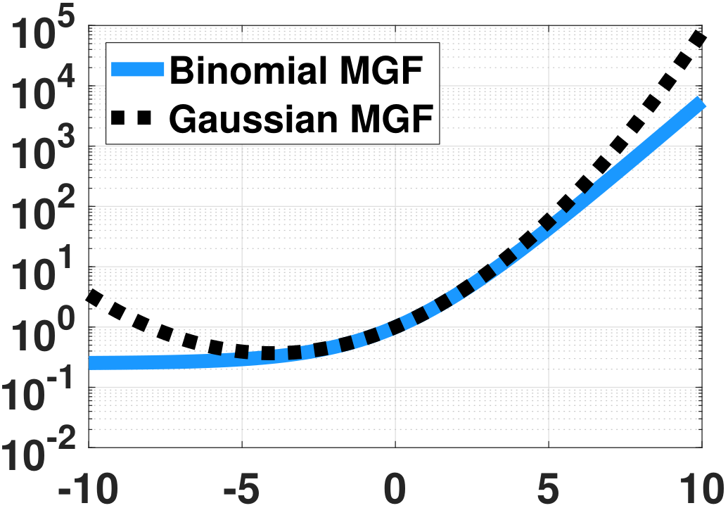
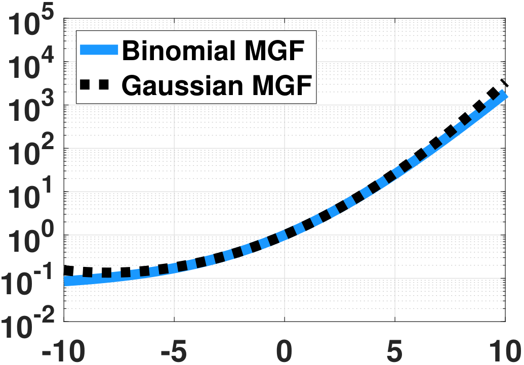
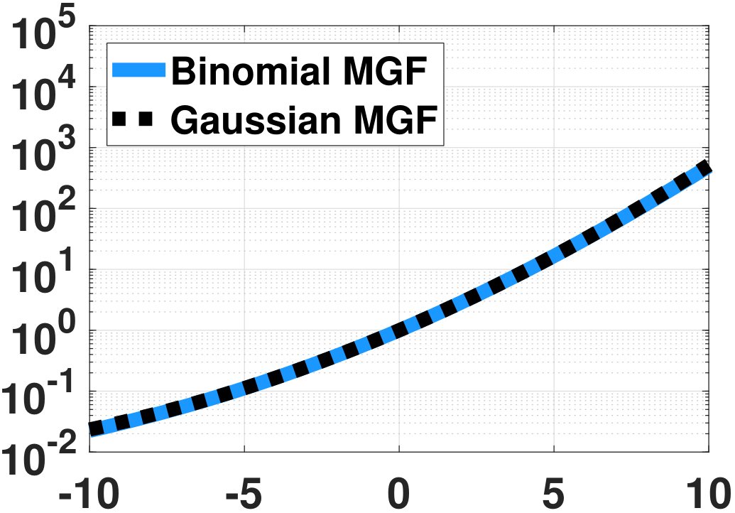
**Figure 6.19.** Explanation of the Central Limit Theorem using the moment-generating function. In this set of plots, we show the MGF of the random variable $\overline{X}_N = (1/N)\sum_{n=1}^NX_n$, where $X_1,\ldots,X_N$ are i.i.d. Bernoulli random variables. The exact MGF of $\overline{X}_N$ is the binomial, whereas the approximated MGF is the Gaussian. We observe that as $N$ increases, the Gaussian approximation to the exact MGF improves.

The reason why the second-order approximation works for Gaussian is that when $N$ increases, the higher order moments of $\overline{X}_N$ vanish and only the leading first two moments survive. The MGFs are becoming flat because $M_Y(s) = \exp\left\{sp + \frac{s^2p(1-p)}{2N}\right\}$ converges to $\exp\{sp\}$ when $N \rightarrow \infty$. Taking the inverse Laplace transform, $M_Y(s) = \exp\{sp\}$ corresponds to a delta function. This makes sense because as $N$ grows, the variance of $\overline{X}_N$ shrinks.

End of the discussion.

6.4.3Examples

Example 6.18

Prove the equivalence of two statements.

sep0ex
$\sqrt{N}\left(\frac{\overline{X}_N-\mu}{\sigma}\right) \overset{d}{\rightarrow} \text{Gaussian}(0,1)$
$\sqrt{N}(\overline{X}_N-\mu) \overset{d}{\rightarrow} \text{Gaussian}(0,\sigma^2)$

Solution

The proof is based on the linear transformation property of Gaussian random variables. For example, if the first statement is true, then the second statement is also true because

\begin{aligned} \lim_{N\rightarrow \infty} F_{\sqrt{N}(\overline{X}_N-\mu)}(z) &= \lim_{N\rightarrow \infty} \Pb[\sqrt{N}(\overline{X}_N-\mu) \le z] \\ &= \lim_{N\rightarrow \infty} \Pb\left[\sqrt{N} \left(\frac{\overline{X}_N-\mu}{\sigma}\right) \le \frac{z}{\sigma}\right]\\ &= \int_{-\infty}^{z/\sigma} \frac{1}{\sqrt{2\pi}} e^{-\frac{t^2}{2}}\;dt= \int_{-\infty}^{z} \frac{1}{\sqrt{2\pi \sigma^2}} e^{-\frac{t^2}{2\sigma^2}}\;dt. \end{aligned}

The other results can be proved similarly.

Example 6.19

Suppose $X_n \sim \mathrm{Poisson}(10)$ for $n = 1,\ldots,N$, and let $\overline{X}_N$ be the sample average. Use the Central Limit Theorem to approximate $\Pb[9 \le \overline{X}_N \le 11]$ for $N = 20$.

Solution

We first show that

\begin{aligned} \E[\overline{X}_N] &= \E\left[\frac{1}{N}\sum_{n=1}^N X_n\right] = \frac{1}{N}\sum_{n=1}^N \E\left[X_n\right] = 10,\\ \Var[\overline{X}_N] &= \frac{1}{N^2}\sum_{n=1}^N \Var\left[X_n\right] = \frac{1}{N}\Var[X_n] = \frac{10}{20} = \frac{1}{2}. \end{aligned}

Therefore, the Central Limit Theorem implies that $\overline{X}_N \overset{d}{\longrightarrow} \text{Gaussian}\left(10,\frac{1}{2}\right)$. The probability is

\begin{aligned} \Pb[9 \le \overline{X}_N \le 11] &\approx \Phi\left( \frac{11-10}{\sqrt{1/2}}\right) - \Phi\left( \frac{9-10}{\sqrt{1/2}}\right)\\ &= \Phi\left( \frac{1}{\sqrt{0.5}}\right) - \Phi\left(-\frac{1}{\sqrt{0.5}}\right) = 0.9214 - 0.0786 = 0.8427. \end{aligned}

We can also do an exact calculation to verify our approximation. Let $S_N = \sum_{n=1}^N X_n$ so that $\overline{X}_N = \frac{S_N}{N}$. Since a sum of Poisson remains a Poisson, it follows that

S_N \sim \text{Poisson}(10N) = \text{Poisson}(200).

Consequently,

\begin{aligned} \Pb[9 \le \overline{X}_N \le 11] &= \Pb[180 \le S_N \le 220] \\ &= \sum_{\ell=0}^{220}\frac{200^\ell e^{-200}}{\ell!} - \sum_{\ell=0}^{180}\frac{200^\ell e^{-200}}{\ell!} = 0.9247 - 0.0822 = 0.8425. \end{aligned}

Note that this is an exact calculation subject to numerical errors when evaluating the finite sums.

Example 6.20

Suppose you have collected $N = 100$ data points from an unknown distribution. The only thing you know is that the true population mean is $\mu = 500$ and the standard deviation is $\sigma = 80$. (Note that this distribution is not necessarily a Gaussian.)

sep0ex
(a) Find the probability that the sample mean will be inside the interval $(490,510)$.
(b) Find an interval such that 95% of the sample average is covered.

Solution

To solve (a), we note that $\overline{X}_N \overset{d}{\rightarrow} \text{Gaussian}\left(500, \left(\tfrac{80}{\sqrt{100}}\right)^2\right)$. Therefore,

\begin{aligned} \Pb[490 \le \overline{X}_N \le 510] &= \Phi\left(\frac{510-500}{\frac{80}{\sqrt{100}}}\right) - \Phi\left(\frac{490-500}{\frac{80}{\sqrt{100}}}\right) \\ &= \Phi(1.25) - \Phi(-1.25) = 0.7888. \end{aligned}

To solve (b), we know that $\Phi(x) = 0.025$ implies that $x = -1.96$, and $\Phi(x) = 0.975$ implies that $x = +1.96$. So

\begin{aligned} \frac{y-500}{\frac{80}{\sqrt{100}}} = \pm 1.96 \quad \Rightarrow \quad y = 484.32 \quad \text{or} \quad y = 515.68. \end{aligned}

Therefore, $\Pb[484.32 \le \overline{X}_N \le 515.68] = 0.95$.

6.4.4Limitation of the Central Limit Theorem

If we recall the statement of the Central Limit Theorem (Berry-Esseen), we observe that the theorem states only that

\lim_{N\rightarrow \infty} \Pb\left[ \sqrt{N} \left( \frac{ \overline{X}_N- \mu}{\sigma}\right) \le \varepsilon \right] = \lim_{N\rightarrow \infty} F_{Z_N}(\varepsilon) = F_Z(\varepsilon) = \Phi(\varepsilon).

Rearranging the terms,

\lim_{N\rightarrow \infty} \Pb\left[ \overline{X}_N \le \mu + \frac{\sigma\varepsilon}{\sqrt{N}} \right] = \Phi(\varepsilon).

This implies that the approximation is good only when the deviation $\varepsilon$ is small.

Let us consider an example to illustrate this idea. Consider a set of i.i.d. exponential random variables $X_1,\ldots,X_N$, where $X_n \sim \text{Exponential}(\lambda)$. Let $S_N = X_1+\cdots+X_N$ be the sum, and let $\overline{X}_N = S_N/N$ be the sample average. Then, according to Chapter 6.4.1, $S_N$ is an Erlang distribution $S_N \sim \text{Erlang}(N,\lambda)$ with a PDF

f_{S_N}(x) = \frac{\lambda^{N}}{(N-1)!} x^{N-1} e^{-\lambda x}.

Practice Exercise 6.10

Let $S_N \sim \text{Erlang}(N,\lambda)$ with a PDF $f_{S_N}(x)$. Show that if $Y_N = aS_N + b$ for any constants $a$ and $b$, then

f_{Y_N}(y) = \frac{1}{a}f_{S_N}\left(\frac{y-b}{a}\right).

Solution

: This is a simple transformation of random variables:

\begin{aligned} F_{Y_N}(y) &= \Pb[Y \le y] = \Pb[aS_N + b \le y] = \Pb\left[S_N \le \frac{y-b}{a}\right]= \int_{-\infty}^{\frac{y-b}{a}} f_{S_N}(x)\;dx. \end{aligned}

Hence, using the fundamental theorem of calculus,

\begin{aligned} f_{Y_N}(y) = \frac{d}{dy} \int_{-\infty}^{\frac{y-b}{a}} f_{S_N}(x)\;dx = \frac{1}{a}f_{S_N}\left(\frac{y-b}{a}\right). \end{aligned}

We are interested in knowing the statistics of $\overline{X}_N$ and comparing it with a Gaussian. To this end, we construct a normalized variable

\begin{aligned} Z_N = \frac{\overline{X}_N-\mu}{\sigma/\sqrt{N}}, \end{aligned}

where $\mu = \E[X_n] = \frac{1}{\lambda}$ and $\sigma^2 = \Var[X_n] = \frac{1}{\lambda^2}$. Then

Z_N = \frac{S_N/N-\mu}{\sigma/\sqrt{N}} = \frac{S_N - N\mu}{\sigma\sqrt{N}} = \frac{\lambda}{\sqrt{N}}S_N - \sqrt{N}

Using the result of the practice exercise, by mapping $a = \frac{\lambda}{\sqrt{N}}$ and $b = -\sqrt{N}$, it follows that

f_{Z_N}(z) = \frac{\sqrt{N}}{\lambda} f_{S_N}\left(\frac{z+\sqrt{N}}{\frac{\lambda}{\sqrt{N}}}\right).

Now we compare $Z_N$ with the standard Gaussian $Z \sim \text{Gaussian}(0,1)$. According to the Central Limit Theorem, the standard Gaussian is a good approximation to the normalized sample average $Z_N$. To compare the two results, we conduct a numerical experiment. We let $\lambda = 1$ and we vary $N$. We plot the PDF $f_{Z_N}(z)$ as a function of $z$, for different $N$'s, in Figure 6.20. In addition, we plot the PDF $f_Z(z)$, which is the standard Gaussian.

The plot in Figure 6.20 shows that while the Central Limit Theorem provides a good approximation, the approximation is only good for values that are close to the mean. For the tails, the Gaussian approximation is not as good.

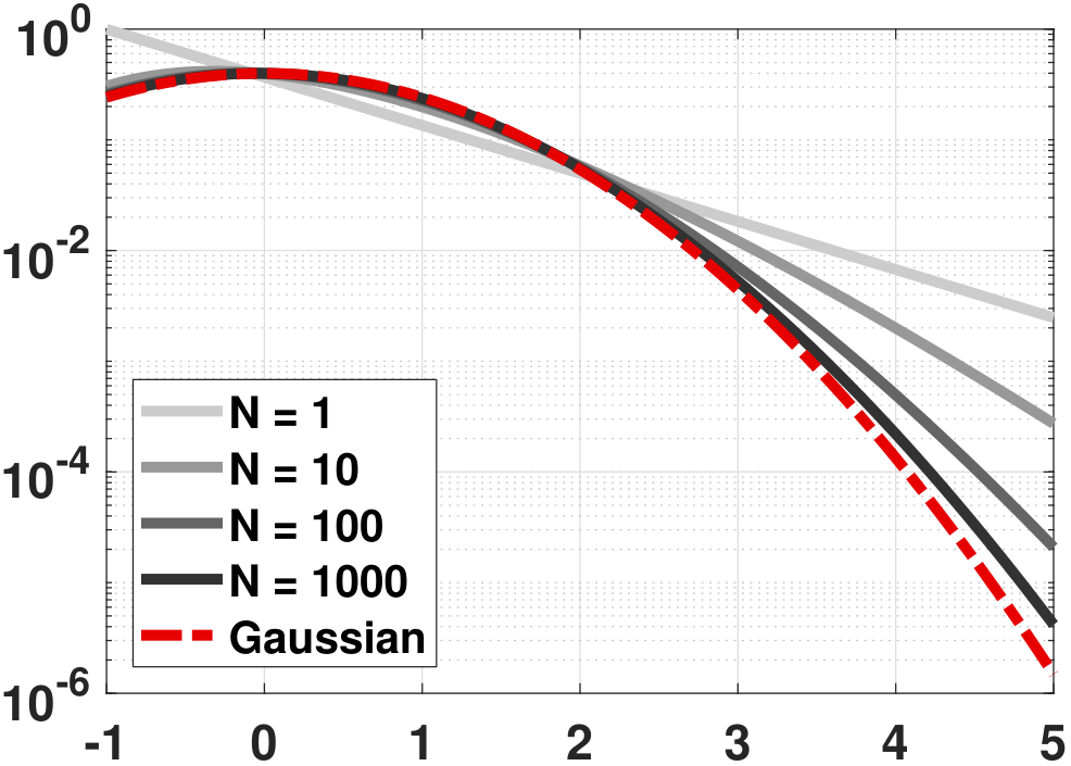
The limitation of the Central Limit Theorem is attributable to the fact that Gaussian is a second-order approximation. If a random variable has a very large third moment, the second-order approximation may not be sufficient. In this case, we need a much larger $N$ to drive the third moment to a small value and make the Gaussian approximation valid.

When will the Central Limit Theorem fail?

sep0ex
The Central Limit Theorem fails when $N$ is small.
The Central Limit Theorem fails if the third moment is large. As an extreme case, a Cauchy random variable does not have a finite third moment. The Central Limit Theorem is not valid for this case.
The Central Limit Theorem can only approximate the probability for input values near the mean. It does not approximate the tails, for which we need to use Chernoff's bound.