eBook › Chapter 7 · Regression

Section 7.2

Overfitting

The regression principle we have discussed in the previous section is a powerful technique for data analysis. However, there are many ways in which things can fall apart. We have seen the problem of outliers, where perturbations of one or a few data points would result in a big change in the regression result, and we discussed some techniques to overcome the outlier problem, e.g., using robust regression. In addition to outliers, there are other causes of the failure of the regression.

In this section, we examine the relationship between the number of training samples and the complexity of the model. For example, if we decide to use polynomials as the basis functions and we have only $N = 20$ data points, what should be the order of the polynomials? Shall we use the 5th-order polynomial, or shall we use the 20th-order polynomial? Our goal in this section is to acquire an understanding of the general problem known as overfitting. Then we will discuss methods for mitigating overfitting in Section sec: ch7 regularization.

7.2.1Overview of overfitting

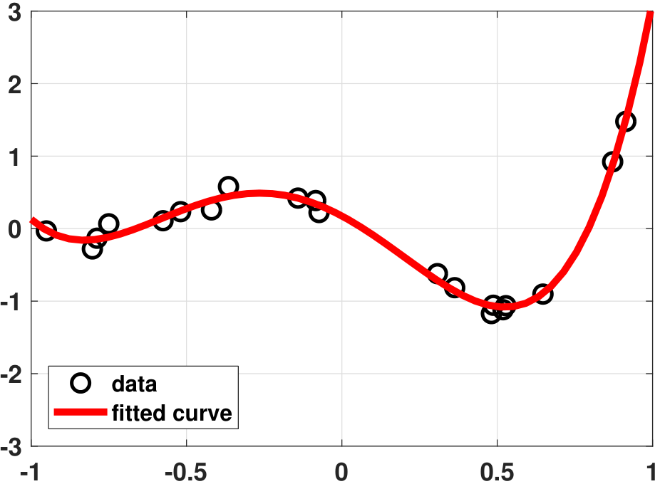
Imagine that we have a dataset containing $N = 20$ training samples. We know that the data are generated from a fourth-order polynomial with Legendre polynomials as the basis. On top of these samples, we also know that a small amount of noise corrupts each sample, for example, Gaussian noise of standard deviation $\sigma = 0.1$.

We have two options here for fitting the data:

sep0ex
Option 1: $h(x) = \sum_{p=0}^4 \theta_p L_p(x)$, which is a 4th-order polynomial.
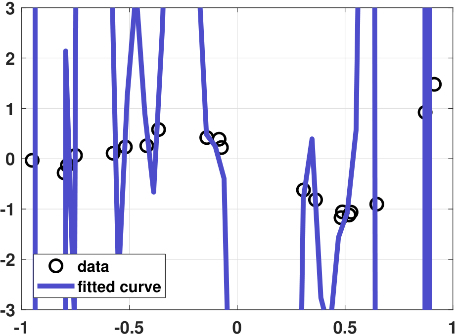
Option 2: $g(x) = \sum_{p=0}^{50} \theta_p L_p(x)$, which is a 50th-order polynomial.

Model 2 is more expressive because it has more degrees of freedom. Let us fit the data using these two models. Figure 7.9 shows the results. However, what is going on with the 50th-order polynomial? It has gone completely wild. How can the regression ever choose such a terrible model?

**Figure 7.9.** Fitting data using a 4th-order polynomial and a 50th-order polynomial.

Here is an even bigger surprise: If we compute the training loss, we get

\begin{aligned} \calE_{\text{train}}(h) &= \frac{1}{N}\sum_{n=1}^N \bigg( y_n - h(x_n) \bigg)^2 = 0.0063,\\ \calE_{\text{train}}(g) &= \frac{1}{N}\sum_{n=1}^N \bigg( y_n - g(x_n) \bigg)^2 = 5.7811 \times 10^{-24}. \end{aligned}

Thus, while Model 2 looks wild in the figure, it has a much lower training loss than Model 1. So according to the training loss, Model 2 fits better.

Any sensible person at this point will object, since Model 2 cannot possibly be better, for the following reason. It is not because it “looks bad”, but because if you test the model with an unseen sample it is almost certain that the testing error will explode. For example, in Figure 7.9(a) if we look at $x = 0$, we would expect the predicted value to be close to $y = 0$. However, Figure 7.9(b) suggests that the predicted value is going to negative infinity. It would be hard to believe that the negative infinity is a better prediction than the other one. We refer to this general phenomenon of fitting very well to the training data but generalizing poorly to the testing data as overfitting.

What is overfitting?

Overfitting means that a model fits too closely to the training samples so that it fails to generalize.

Overfitting occurs as a consequence of an imbalance between the following three factors:

sep0ex
Number of training samples $N$. If you have many training samples, you should learn very well, even if the model is complex. Conversely, if the model is complex but does not have enough training samples, you will overfit it. The most serious problem in regression is often insufficient training data.
Model order $d$. This refers to the complexity of the model. For example, if your model uses a polynomial, $d$ refers to the order of the polynomial. If your training set is too small, you need to use a less complex model. The general rule of thumb is: “less is more”.
Noise variance $\sigma^2$. This refers to the variance of the error $e_n$ you add to the data. The model we assumed in the previous numerical experiment is that
$y_n = g(x_n) + e_n, \qquad n = 1,\ldots,N.$
where $e_n \sim \text{Gaussian}(0,\sigma^2)$. If $\sigma$ increases, it is inevitable that the fitting will become more difficult. Hence fitting would require more training samples, and perhaps a less complex model would work better.

7.2.2Analysis of the linear case

Let us spell out the details of these factors one by one. To make our discussion concrete, we will use linear regression as a case study. The general analysis will be presented in the next section.

Notations

sep0ex
Ground Truth Model. To start with, we assume that we have a population set $\calD$ containing infinitely many samples $(\vx,y)$ drawn according to some latent distributions. The relationship between $\vx$ and $y$ is defined through an unknown target function
$y = f(\vx) + e,$
where $e \sim \text{Gaussian}(0,\sigma^2)$ is the noise. For our analysis, we assume that $f(\cdot)$ is linear, so that
$f(\vx) = \vx^T\vtheta^*,$
where $\vtheta^* \in \R^d$ is the ground truth model parameter. Notice that $f(\cdot)$ is deterministic, but $e$ is random. Therefore, any randomness we see in $y$ is due to $e$.
Training and Testing Set. From $\calD$, we construct two datasets: the training data set $\calD_{\text{train}}$ that contains training samples $\{(\vx_1,y_1),\ldots,(\vx_N,y_N)\}$ and the testing dataset $\calD_{\text{test}}$ that contains $\{(\vx_1,y_1),\ldots,(\vx_M,y_M)\}$. Both $\calD_{\text{train}}$ and $\calD_{\text{test}}$ are subsets of $\calD$.
Predictive Model. We consider a predictive model $g_{\vtheta}(\cdot)$. For simplicity, we assume that $g_{\vtheta}(\cdot)$ is also linear:
$g_{\vtheta}(\vx) = \vx^T\vtheta.$
Given the training dataset $\calD = \{(\vx_1,y_1),\ldots,(\vx_N,y_N)\}$, we construct a linear regression problem:
$\vthetahat = \argmin{\vtheta \in \R^d} \;\; \|\mX\vtheta - \vy\|^2.$
Throughout our analysis, we assume that $N \ge d$ so that we have more training data than the number of unknowns. We further assume that $\mX^T\mX$ is invertible, and so there is a unique global minimizer
$\vthetahat = (\mX^T\mX)^{-1}\mX^T\vy.$
Training Error. Given the estimated model parameter $\vthetahat$, we define the in-sample prediction as
$\vyhat_{\text{train}} = \mX_{\text{train}}\vthetahat,$
where $\mX_{\text{train}} = \mX$ is the training data matrix. The in-sample prediction is the predicted value using the trained model for the training data. The corresponding error with respect to the ground truth is called the training error:
$\calE_{\text{train}}(\vthetahat) = \E_{\ve} \left[ \frac{1}{N} \|\vyhat_{\text{train}} - \vy\|^2\right],$
where $N$ is the number of training samples in the training dataset. Note that the expectation is taken with respect to the noise vector $\ve$, which follows the distribution $\text{Gaussian}(0, \sigma^2\mI)$.
Testing Error. During testing, we construct a testing matrix $\mX_{\text{test}}$. This gives us the estimated values $\vyhat_{\text{test}}$:
$\vyhat_{\text{test}} = \mX_{\text{test}}\vthetahat.$
The out-of-sample prediction is the predicted value using the trained model for the testing data. The corresponding error with respect to the ground truth is called the testing error:
$\calE_{\text{test}}(\vthetahat) = \E_{\ve} \left[ \frac{1}{M} \|\vyhat_{\text{test}} - \vy\|^2 \right],$
where $M$ is the number of testing samples in the testing dataset.

Analysis of the training error

We first analyze the training error, which we defined as

\begin{aligned} \calE_{\text{train}} &= \E_{\ve}\bigg[ \frac{1}{N}\left\|\vyhat - \vy \right\|^2\bigg] \bydef \text{MSE}(\vyhat, \vy). \end{aligned}

For this particular choice of the training error, we call it the mean squared error (MSE). It measures the difference between $\vyhat$ and $\vy$.

Theorem 7.3

Let $\vtheta^* \in \R^d$ be the ground truth linear model parameter, and $\mX \in \R^{N \times d}$ be a matrix such that $N \ge d$ and $\mX^T\mX$ is invertible. Assume that the data follows the linear model $\vy = \mX\vtheta^* + \ve$ where $\ve \sim \text{Gaussian}(0,\sigma^2\mI)$. Consider the linear regression problem $\vthetahat = \argmin{\vtheta \in \R^d} \; \|\mX\vtheta-\vy\|^2$, and the predicted value $\vyhat = \mX\vthetahat$. The mean squared training error of this linear model is

\calE_{\text{train}} \bydef \text{MSE}(\vyhat, \vy) = \E_{\ve}\bigg[ \frac{1}{N} \left\|\vyhat - \vy \right\|^2\bigg] = \sigma^2\left(1-\frac{d}{N}\right).

The proof below depends on some results from linear algebra that may be difficult for first-time readers. We recommend you read the proof later.

Proof. Recall that the least squares linear regression solution is $\vthetahat = (\mX^T\mX)^{-1}\mX^T\vy$. Since $\vy = \mX\vtheta^* + \ve$, we can substitute this into the predicted value $\vyhat$ to show that

\begin{aligned} \vyhat = \mX\vthetahat &= \underset{=\textcolor{black}{\mH}}{\underbrace{\mX(\mX^T\mX)^{-1}\mX^T}}\vy = \mX(\mX^T\mX)^{-1}\mX^T(\mX\vtheta^* + \ve) = \mX\vtheta^* + \mH\ve. \end{aligned}

Therefore, substituting $\vyhat = \mX\vtheta^* + \mH\ve$ into the MSE,

\begin{aligned} \text{MSE}(\vyhat, \vy) \bydef \E_{\ve}\bigg[ \frac{1}{N} \left\|\vyhat - \vy \right\|^2\bigg] &= \E_{\ve}\bigg[ \frac{1}{N} \left\|\mX\vtheta^* + \mH\ve - \mX\vtheta^* - \ve \right\|^2\bigg]\\ &= \E_{\ve}\bigg[ \frac{1}{N} \left\| (\mH-\mI)\ve\right\|^2\bigg]. \end{aligned}

At this point we need to use a tool from linear algebra. One useful identity{The reason for this identity is that

\begin{aligned} \|\vv\|^2 = \sum_{n=1}^N v_n^2 = \text{Tr} \left\{ \begin{bmatrix} \textcolor{black}{v_1^2} & v_1v_2 & \cdots & v_1v_N\\ v_2v_1 & \textcolor{black}{v_2^2} & \cdots & v_2v_N\\ \vdots & \vdots & \textcolor{black}{\ddots} & \vdots\\ v_Nv_1 & v_Nv_2 & \cdots & \textcolor{black}{v_N^2} \end{bmatrix} \right\} = \text{Tr}\left\{\vv\vv^T\right\}. \end{aligned}

} is that for any $\vv \in \R^N$,

\begin{aligned} \|\vv\|^2 = \text{Tr}(\vv\vv^T). \end{aligned}

Using this identity, we have that

\begin{aligned} \E_{\ve}\bigg[ \frac{1}{N} \left\| (\mH-\mI)\ve\right\|^2\bigg] &= \frac{1}{N} \E_{\ve}\bigg[ \text{Tr}\bigg\{ (\mH-\mI)\ve \ve^T(\mH-\mI)^T \bigg\} \bigg] \\ &= \frac{1}{N} \text{Tr}\bigg\{ (\mH-\mI) \textcolor{black}{\E_{\ve}\big[\ve \ve^T\big]}(\mH-\mI)^T \bigg\} \\ &= \frac{\sigma^2}{N} \text{Tr}\bigg\{ (\mH-\mI)(\mH-\mI)^T \bigg\}, \end{aligned}

where we used the fact that $\E[\ve\ve^T] = \sigma^2\mI$. The special structure of $\mH$ tells us that $\mH^T = \mH$ and $\mH^T\mH = \mH$. Thus, we have $(\mH-\mI)^T(\mH-\mI) = \mI-\mH$. In addition, using the cyclic property of trace $\text{Tr}(\mA\mB) = \text{Tr}(\mB\mA)$, we have that

\begin{aligned} \text{Tr}(\mH) &= \text{Tr}(\mX(\mX^T\mX)^{-1}\mX^T) \\ &= \text{Tr}((\mX^T\mX)^{-1}\mX^T\mX) = \text{Tr}(\mI) = d. \end{aligned}

Consequently,

\begin{aligned} \frac{\sigma^2}{N} \text{Tr}\bigg\{ (\mH-\mI)(\mH-\mI)^T \bigg\} &= \frac{\sigma^2}{N} \text{Tr}\bigg\{ \mI-\mH \bigg\} \\ &= \sigma^2\left(1-\frac{d}{N}\right). \end{aligned}

This completes the proof.

■

The end of the proof. Please join us again.

Practice Exercise 1

In the theorem above, we proved the MSE of the prediction $\vyhat$. In this example, we would like to prove the MSE for the parameter. Prove that

\begin{aligned} \text{MSE}(\vthetahat, \vtheta^*) &\bydef \E_{\ve}\bigg[ \left\|\vthetahat - \vtheta^* \right\|^2\bigg] = \sigma^2 \text{Tr} \bigg\{(\mX^T\mX)^{-1}\bigg\}. \end{aligned}

Solution

Let us start with the definition:

\begin{aligned} \text{MSE}(\vthetahat, \vtheta^*) &= \E_{\ve}\bigg[ \left\|(\mX^T\mX)^{-1}\mX^T\vy - \vtheta^* \right\|^2\bigg]\\ &= \E_{\ve}\bigg[ \left\|(\mX^T\mX)^{-1}\mX^T(\mX\vtheta^*+\ve) - \vtheta^* \right\|^2\bigg]\\ &= \E_{\ve}\bigg[ \left\|\vtheta^*+(\mX^T\mX)^{-1}\mX^T\ve - \vtheta^* \right\|^2\bigg] = \E_{\ve}\bigg[ \left\| (\mX^T\mX)^{-1}\mX^T\ve \right\|^2\bigg]. \end{aligned}

Continuing the calculation,

\begin{aligned} &\E_{\ve}\bigg[ \left\| (\mX^T\mX)^{-1}\mX^T\ve \right\|^2 \bigg] = \E_{\ve}\bigg[ \text{Tr} \bigg\{(\mX^T\mX)^{-1} \mX^T \ve \;\;\; \ve^T \mX (\mX^T\mX)^{-1} \bigg\} \bigg] \\ &= \text{Tr} \bigg\{(\mX^T\mX)^{-1} \mX^T \textcolor{black}{\E_{\ve}\bigg[ \ve \ve^T \bigg]} \mX (\mX^T\mX)^{-1}\bigg\} \\ &= \text{Tr} \bigg\{(\mX^T\mX)^{-1} \mX^T \;\cdot\; \textcolor{black}{\sigma^2\mI} \;\cdot\; \mX (\mX^T\mX)^{-1}\bigg\} \\ &= \sigma^2 \text{Tr} \bigg\{(\mX^T\mX)^{-1} \mX^T \;\cdot\; \mX (\mX^T\mX)^{-1}\bigg\} = \sigma^2 \text{Tr} \bigg\{(\mX^T\mX)^{-1}\bigg\}. \end{aligned}

Analysis of the testing error

Similarly to the training error, we can analyze the testing error. The testing error is defined as

\calE_{\text{test}} = \text{MSE}(\vyhat,\vy') \bydef \E_{\ve,\ve'}\bigg[ \frac{1}{M}\left\|\vyhat - \vy' \right\|^2\bigg],

where $\vyhat = [\yhat_1,\ldots,\yhat_M]^T$ is a vector of $M$ predicted values and $\vy' = [y_1',\ldots,y_M']^T$ is a vector of $M$ true values in the testing data. (In practice, the number of testing samples $M$ can be much larger than the number of training samples $N$. This probably does not agree with your experience, in which the testing dataset is often much smaller than the training dataset. The reason for this paradox is that the practical testing data set is only a finite subset of all the possible testing samples available. So the “testing error” we compute in practice approximates the true testing error. If you want to compute the true testing error, you need a very large testing dataset.)

We would like to derive something concrete. To make our analysis simple, we consider a special case in which the testing set contains $(x_1,y_1'),\ldots,(x_N,y_N')$. That is, the inputs $x_1,\ldots,x_N$ are identical for both training and testing (for example, suppose that you measure the temperature on two different days but at the same time stamps.) In this case, we have $M = N$, and we have $\mX_{\text{test}} = \mX_{\text{train}} = \mX$. However, the noise added to the testing data is still different from the noise added to the training data.

With these simplifications, we can derive the testing error as follows.

Theorem 7.4

Let $\vtheta^* \in \R^d$ be the ground truth linear model parameter, and $\mX \in \R^{N \times d}$ be a matrix such that $N \ge d$ and $\mX^T\mX$ is invertible. Assume that the training data follows the linear model $\vy = \mX\vtheta^* + \ve$, where $\ve \sim \text{Gaussian}(0,\sigma^2\mI)$. Consider the linear regression problem $\vthetahat = (\mX^T\mX)^{-1}\mX^T\vy$, and let $\vyhat = \mX\vthetahat$. Let $\mX_{\text{test}} = \mX$ be the testing input data matrix, and define $\vy' = \mX_{\text{test}}\vtheta^* + \ve' \in \R^N$, with $\ve' \sim \text{Gaussian}(0,\sigma^2\mI)$, be the testing output. Then, the mean squared testing error of this linear model is

\calE_{\text{test}} \bydef \text{MSE}(\vyhat, \vy') = \E_{\ve,\ve'}\bigg[ \frac{1}{N} \left\|\vyhat - \vy' \right\|^2\bigg] = \sigma^2\left(1+\frac{d}{N}\right).

In this definition, the expectation is taken with respect to a joint distribution of $(\ve,\ve')$. This is because, in testing, the trained model is based on $\vy$ of which the randomness is $\ve$. However, the testing data is based on $\vy'$, where the randomness comes from $\ve'$. We assume that $\ve$ and $\ve'$ are independent i.i.d. Gaussian vectors.

As with the previous proof, we recommend you study this proof later.

Proof. The MSE can be derived from the definition:

\begin{aligned} \text{MSE}(\vyhat, \vy') &= \E_{\ve,\ve'}\bigg[ \frac{1}{N} \left\|\vyhat - \vy' \right\|^2\bigg] \\ &= \frac{1}{N} \E_{\ve,\ve'}\bigg[ \left\|\mX\vtheta^* + \mH\ve - \mX\vtheta^* - \ve' \right\|^2\bigg]\\ &= \frac{1}{N} \E_{\ve,\ve'}\bigg[ \left\|\mH\ve - \ve' \right\|^2\bigg]. \end{aligned}

Since each noise term $e_n$ and $e_n'$ is an i.i.d. copy of the same Gaussian random variable, by using the fact that

\begin{aligned} \text{Tr}(\mH) &= \text{Tr}(\mX(\mX^T\mX)^{-1}\mX^T) \\ &= \text{Tr}((\mX^T\mX)^{-1}\mX^T\mX) = \text{Tr}(\mI) = d, \end{aligned}

we have that

\begin{aligned} \E_{\ve,\ve'} \left[ \left\|\mH\ve - \ve' \right\|^2 \right] &= \E_{\ve} \left[\|\mH\ve\|^2\right] - \underset{=0}{\underbrace{\E_{\ve,\ve'} \left[2\ve^T\mH^T\ve'\right]}} + \E_{\ve'} \left[\|\ve'\|^2\right]\\ &= \E_{\ve}\left[ \text{Tr} \left\{\mH \ve \ve^T \mH^T\right\}\right] + \E_{\ve'}\left[ \text{Tr}\left\{\ve' \ve'^{T}\right\}\right]\\ &= \text{Tr} \left\{\mH \E_{\ve}\left[\ve \ve^T\right] \mH^T\right\} + \text{Tr}\{\E_{\ve'}\left[\ve' \ve'^{T}\right]\}\\ &= \text{Tr} \left\{\mH \cdot \sigma^2\mI_{N \times N} \cdot \mH^T\right\} + \text{Tr}\left\{\sigma^2 \mI_{N \times N}\right\}\\ &= \sigma^2 \text{Tr} \left\{\mH \mH^T\right\} + \text{Tr}\left\{\sigma^2 \mI_{N \times N}\right\}\\ &= \sigma^2 \text{Tr}(\mI_{d \times d}) + \sigma^2 \text{Tr}\left\{\mI_{N \times N}\right\} = \sigma^2(d+N). \end{aligned}

Combining all the terms,

\begin{aligned} \text{MSE}(\vyhat, \vy') = \E_{\ve,\ve'}\bigg[ \frac{1}{N} \left\|\vyhat - \vy' \right\|^2\bigg] = \sigma^2\left(1+\frac{d}{N}\right), \end{aligned}

which completes the proof.

■

The end of the proof.

7.2.3Interpreting the linear analysis results

Let us summarize the two main theorems. They state that, for $N \ge d$,

\begin{aligned} \calE_{\text{train}} &\bydef \text{MSE}(\vyhat, \vy) = \E_{\ve}\bigg[ \frac{1}{N} \left\|\vyhat - \vy \right\|^2\bigg] = \sigma^2\left(1-\frac{d}{N}\right),\\ \calE_{\text{test}} &\bydef \text{MSE}(\vyhat, \vy') = \E_{\ve,\ve'}\bigg[ \frac{1}{N} \left\|\vyhat - \vy' \right\|^2\bigg] = \sigma^2\left(1+\frac{d}{N}\right). \end{aligned}

This pair of equations tells us everything about the overfitting issue.

How do $\calE_{{train

}$and$\calE_test$change w.r.t.~$^2$?}

sep0ex
$\calE_{\text{train}}$ $\uparrow$ as $\sigma^2$ $\uparrow$. Thus noisier data are harder to fit.
$\calE_{\text{test}}$ $\uparrow$ as $\sigma^2$ $\uparrow$. Thus a noisier model is more difficult to generalize.

The reasons for these results should be clear from the following equations:

\begin{aligned} \calE_{\text{train}} &= \textcolor{red}{\sigma^2}\left(1-\frac{d}{N}\right),\\ \calE_{\text{test}} &= \textcolor{red}{\sigma^2}\left(1+\frac{d}{N}\right). \end{aligned}

As $\sigma^2$ increases, the training error $\calE_{\text{train}}$ grows linearly w.r.t. $\sigma^2$. Since the training error measures how good your model is compared with the training data, a larger $\calE_{\text{train}}$ means it is more difficult to fit. For the testing case, $\calE_{\text{test}}$ also grows linearly w.r.t. $\sigma^2$. This implies that the model would be more difficult to generalize if the model were trained using noisier data.

How do $\calE_{{train

}$and$\calE_test$change w.r.t.~$N$?}

sep0ex
$\calE_{\text{train}}$ $\uparrow$ as $N$ $\uparrow$. Thus more training samples make fitting harder.
$\calE_{\text{test}}$ $\downarrow$ as $N$ $\uparrow$. Thus more training samples improve generalization.

The reason for this should also be clear from the following equations:

\begin{aligned} \calE_{\text{train}} &= \sigma^2\left(1-\frac{d}{\textcolor{red}{N}}\right),\\ \calE_{\text{test}} &= \sigma^2\left(1+\frac{d}{\textcolor{red}{N}}\right). \end{aligned}

As $N$ increases, the model sees more training samples. The goal of the model is to minimize the error with all the training samples. Thus the more training samples we have, the harder it will be to make everyone happy; so the training error grows as $N$ grows. For testing, if the model is trained with more samples it is more resilient to noise. Hence the generalization improves.

How do $\calE_{{train

}$and$\calE_test$change w.r.t.~$d$?}

sep0ex
$\calE_{\text{train}}$ $\downarrow$ as $d$ $\uparrow$. Thus a more complex model makes fitting easier.
$\calE_{\text{test}}$ $\uparrow$ as $d$ $\uparrow$. Thus a more complex model makes generalization harder.

These results are perhaps less obvious than the others. The following equations tell us that

\begin{aligned} \calE_{\text{train}} &= \sigma^2\left(1 \textcolor{red}{-}\frac{\textcolor{red}{d}}{N}\right), \\ \calE_{\text{test}} &= \sigma^2\left(1 \textcolor{red}{+}\frac{\textcolor{red}{d}}{N}\right). \end{aligned}

For this linear regression model to work, $d$ has to be less than $N$; otherwise, the matrix inversion $(\mX^T\mX)^{-1}$ is invalid. However, as $d$ grows while $N$ remains fixed, we ask the linear regression to fit a larger and larger model while not providing any additional training samples. Eq. (7.23) says that $\calE_{\text{train}}$ will drop as $d$ increases but $\calE_{\text{test}}$ will increase as $d$ increases. Therefore, a larger model will not generalize as well if $N$ is fixed.

If $d > N$, then the optimization

\vthetahat = \argmin{\vtheta \in \R^d} \;\; \|\mX\vtheta - \vy\|^2

will have many global minimizers (see Figure 7.6), implying that the training error can go to zero. Our analysis of $\calE_{\text{train}}$ and $\calE_{\text{test}}$ does not cover this case because our proofs require $(\mX^T\mX)^{-1}$ to exist. However, we can still extrapolate what will happen. When the training error is zero, it only means that we fit perfectly into the training data. Since the testing error grows as $d$ grows (though not in the particular form shown in Eq. (7.23)), we should expect the testing error to become worse.

Learning curve

The results we derived above can be summarized in the learning curve shown in Figure 7.10. In this figure we consider a simple problem where

y_n = \theta_0 + \theta_1 x_n + e_n,

for $e_n \sim \text{Gaussian}(0,1)$. Therefore, according to our theoretical derivations, we have $\sigma = 1$ and $d = 2$. For every $N$, we compute the average training error $\calE_{\text{train}}$ and the average testing error $\calE_{\text{test}}$, and then mark them on the figure. These are our empirical training and testing errors. On the same figure, we calculate the theoretical training and testing error according to Eq. (7.23).

The MATLAB and Python codes used to generate this learning curve are shown below.

MATLAB

Nset = round(logspace(1,3,20));
    E_train = zeros(1,length(Nset));
    E_test  = zeros(1,length(Nset));
    a = [1.3, 2.5];
    for j = 1:length(Nset)
        N = Nset(j);
        x = linspace(-1,1,N)';
        E_train_temp = zeros(1,1000);
        E_test_temp  = zeros(1,1000);
        X = [ones(N,1), x(:)];
        for i = 1:1000
            y  = a(1) + a(2)*x + randn(size(x));
            y1 = a(1) + a(2)*x + randn(size(x));
            theta = X\y(:);
            yhat = theta(1) + theta(2)*x;
            E_train_temp(i) = mean((yhat(:)-y(:)).^2);
            E_test_temp(i)  = mean((yhat(:)-y1(:)).^2);
        end
        E_train(j) = mean(E_train_temp);
        E_test(j)  = mean(E_test_temp);
    end
    semilogx(Nset, E_train, 'kx', 'LineWidth', 2, 'MarkerSize', 16); hold on;
    semilogx(Nset, E_test, 'ro', 'LineWidth', 2, 'MarkerSize', 8);
    semilogx(Nset, 1-2./Nset, 'k', 'LineWidth', 4);
    semilogx(Nset, 1+2./Nset, 'r', 'LineWidth', 4);

Python

import numpy as np
    import matplotlib.pyplot as plt
    
    Nset = np.logspace(1,3,20)
    Nset = Nset.astype(int)
    E_train = np.zeros(len(Nset))
    E_test  = np.zeros(len(Nset))
    for j in range(len(Nset)):
      N = Nset[j]
      x = np.linspace(-1,1,N)
      a = np.array([1, 2])
      E_train_tmp = np.zeros(1000)
      E_test_tmp  = np.zeros(1000)
      for i in range(1000):
        y              = a[0] + a[1]*x + np.random.randn(N)
        X              = np.column_stack((np.ones(N), x))
        theta          = np.linalg.lstsq(X, y, rcond=None)[0]
        yhat           = theta[0] + theta[1]*x
        E_train_tmp[i] = np.mean((yhat-y)**2)
        y1             = a[0] + a[1]*x + np.random.randn(N)
        E_test_tmp[i]  = np.mean((yhat-y1)**2)
      E_train[j] = np.mean(E_train_tmp)
      E_test[j]  = np.mean(E_test_tmp)
    plt.semilogx(Nset, E_train, 'kx')
    plt.semilogx(Nset, E_test, 'ro')
    plt.semilogx(Nset, (1-2/Nset), linewidth=4, c='k')
    plt.semilogx(Nset, (1+2/Nset), linewidth=4, c='r')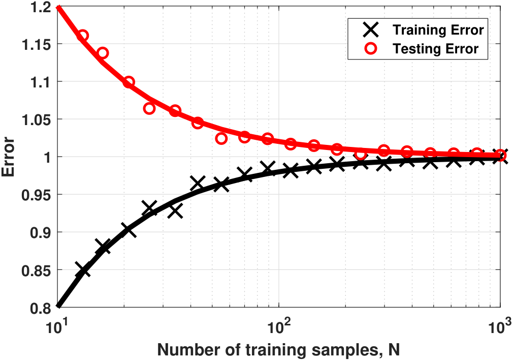

**Figure 7.10.** The learning curve is a pair of functions representing the training error and the testing error. As $N$ increases we expect the training error to increase and the testing error to decrease. The two functions will converge to the same value as $N$ goes to infinity. If they do not converge to the same value, there is an intrinsic mismatch between the training samples and the testing samples, e.g., the training samples are not representative enough for the dataset.

The training error curve and the testing error curve behave in opposite ways as $N$ increases. The training error $\calE_{\text{train}}$ increases as $N$ increases, because when we have more training samples it becomes harder for the model to fit all the data. By contrast, the testing error $\calE_{\text{test}}$ decreases as $N$ increases, because when we have more training samples the model becomes more robust to noise and unseen data. Therefore, the testing error improves.

As $N$ goes to infinity, both the training error and the testing error converge. This is due to the law of large numbers, which says that the empirical training and testing errors should converge to their respective expected values. If the training error and the testing error converge to the same value, the training can generalize to testing. If they do not converge to the same value, there is a mismatch between the training samples and the testing samples.

It is important to pay attention to the gap between the converged values. We often assume that the training samples and the testing samples are drawn from the same distribution, and therefore the training samples are good representatives of the testing samples. If the assumption is not true, there will be a gap between the converged training error and the testing error. Thus, what you claim in training cannot be transferred to the testing. Consequently, the learning curve provides you with a useful debugging tool to check how well your training compares with your testing.

Closing remark. In this section we have studied a very important concept in regression, overfitting. We emphasize that overfitting is not only caused by the complexity of the model but a combination of the three factors $\sigma^2$, $N$, and $d$. We close this section by summarizing the causes of overfitting:

What is the source of overfitting?

sep0ex
Overfitting occurs because you have an imbalance between $\sigma^2$, $N$ and $d$.
Selecting the correct complexity for your model is the key to avoid overfitting.