Regularization
Having discussed the source of the overfitting problem, we now discuss methods to alleviate overfitting. The method we focus on here is regularization. Regularization means that instead of seeking the model parameters by minimizing the training loss alone, we add a penalty term to force the parameters to “behave better”. As a preview of the technique, we change the original training loss
which consists of only the data fidelity term, to a modified training loss
Putting this into the matrix form, we define the data fidelity term as
The newly added term \(R(\vtheta)\) is called the regularization function or the penalty function. It can take a variety of forms, e.g.,
- sep0ex
- Ridge regression: \(R(\vtheta) = \sum_{p=0}^{d-1} \theta_p^2 = \|\vtheta\|^2\).
- LASSO regression: \(R(\vtheta) = \sum_{p=0}^{d-1} |\theta_p| = \|\vtheta\|_1\).
In this section we aim to understand the role of the regularization functions by studying these two examples of \(R(\vtheta)\).
7.4.1Ridge regularization
To explain the meaning of Eq. (7.34) we write it in terms of matrices and vectors:
where \(\lambda\) is called the regularization parameter. It needs to be tuned by the user. We refer to Eq. (7.36) as the ridge regression. (In signal processing and optimization, Eq. (7.36) is called the Tikhonov regularization. We follow the statistics community in calling it the ridge regression.)
How can the regularization function help to mitigate the overfitting problem? First let's find the solution to this problem.
Prove that the solution to Eq. (7.36) is
Take the derivative with respect to \(\vtheta\). (The solution here requires some basic matrix calculus. You may refer to the University of Waterloo's Matrix Cookbook https://www.math.uwaterloo.ca/ hwolkowi/matrixcookbook.pdf.) This yields
Rearranging the terms gives
Inverting the matrix on the left-hand side yields the solution.
Let us compare the ridge regression solution with the vanilla regression solutions:
Clearly, the only difference is the presence of the parameter \(\lambda\):
- sep0ex
If \(\lambda \rightarrow 0\), then \(\vthetahat_{\text{ridge}}(0) = \vthetahat_{\text{vanilla}}\). This is because
$$\calE_{\text{train}}(\vtheta) = \|\mX\vtheta - \vy\|^2 + \underset{=0}{\underbrace{\lambda \|\vtheta\|^2}}.$$Hence, when \(\lambda \rightarrow 0\), the regression problem goes back to the vanilla version, and so does the solution.
If \(\lambda \rightarrow \infty\), then \(\vthetahat_{\text{ridge}}(\infty) = 0\). This happens because
$$\calE_{\text{train}}(\vtheta) = \underset{=0}{\underbrace{\frac{1}{\lambda}\|\mX\vtheta - \vy\|^2}} + \|\vtheta\|^2.$$Since we are now minimizing \(\|\vtheta\|^2\), the solution will be \(\vtheta = 0\) because zero is the smallest value a squared function can achieve.
For any \(0 < \lambda < \infty\), the net effect of \((\mX^T\mX + \lambda \mI)\) is the constant \(\lambda\) added to all the eigenvalues of \(\mX^T\mX\). By taking the eigendecomposition of \(\mX^T\mX\),
we have that
Therefore, if the eigenvalue matrix \(\mS\) has a zero eigenvalue it will be offset by \(\lambda\):
As a result, even if \(\mX^T\mX\) is not invertible (or close to not invertible), the new matrix \(\mX^T\mX+\lambda\mI\) is guaranteed to be invertible.
You may be wondering what happens if \(\mX^T\mX\) has a negative eigenvalue so that when we add a positive \(\lambda\), the resulting matrix may have a zero eigenvalue. Prove that \(\mX^T\mX\) will never have a negative eigenvalue, and \(\mX^T\mX+\lambda\mI\) always has positive eigenvalues.
Eigenvalues of a matrix \(\mA\) are nonnegative if and only if \(\vv^T\mA\vv \ge 0\) for any \(\vv\). Thus we need to check whether \(\vv^T\mX^T\mX\vv \ge 0\) for all \(\vv\). However, this is easy:
which must be nonnegative for any \(\vv\). Matrices satisfying this property are called positive semidefinite. Therefore, \(\mX^T\mX\) is positive semidefinite.
Implementation
Solving the ridge regression is easy. First, we observe that the regularization function \(R(\vtheta) = \|\vtheta\|^2\) is a quadratic function. Therefore, it can be combined with the data fidelity term as
Therefore, all we need to do is to concatenate the matrix \(\mX\) with a \(d \times d\) identity operator \(\sqrt{\lambda}\mI\), and concatenate \(\vy\) with a \(d \times 1\) all-zero vector.
In MATLAB and Python, the implementation of the ridge regression is done by defining a new matrix A and a new vector b, as shown below:
% MATLAB command for ridge regression
    A = [X; sqrt(lambda)*eye(d)];
    b = [y(:); zeros(d,1)];
theta = A\b;% MATLAB command for ridge regression
A = np.vstack((X, np.sqrt(lambd)*np.eye(d)))
b = np.hstack((y, np.zeros(d)))
theta = np.linalg.lstsq(A, b, rcond=None)[0]Consider a dataset of \(N = 20\) data points. These data points are constructed from the model
where \(e_n \sim \text{Gaussian}(0,0.25^2)\) is the noise. Fit the data using
- sep0ex
- (a) Vanilla linear regression with a \(4\)th-order polynomial.
- (b) Vanilla linear regression with a 20th-order polynomial.
- (c) Ridge regression with a 20th-order polynomial, by considering three choices of \(\lambda\): \(\lambda = 10^{-6}\), \(\lambda = 10^{-3}\), and \(\lambda = 10\).
- sep0ex
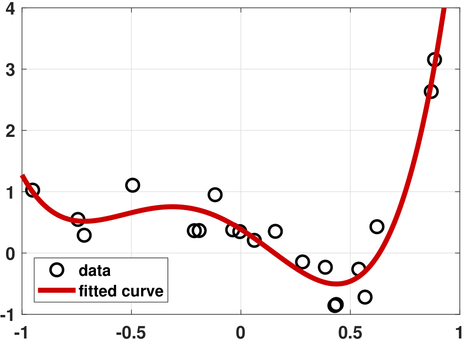
- (a) We first fit the data using a 4th-order polynomial. This fitting is relatively straightforward. In the MATLAB / Python programs below, set \(d = 4\) and \(\lambda = 0\). The result is shown in Figure 7.16(a).
- sep0ex
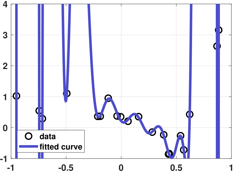
- (b) Suppose we use a 20th-order polynomial \(g(x) = \sum_{p=0}^{20} \theta_p x^p\) to fit the data. We plot the result in Figure 7.16(b). Since the order of the polynomial is very high relative to the number of training samples, it comes as no surprise that the fitting is poor. This is overfitting, and we know the reason.
- sep0ex
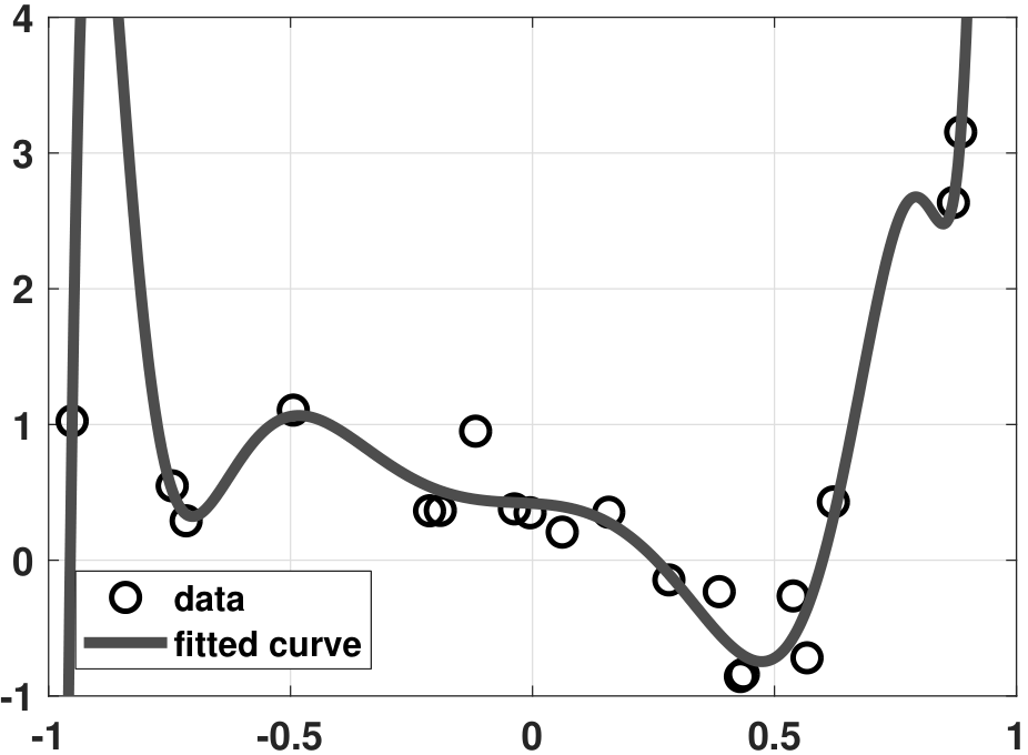
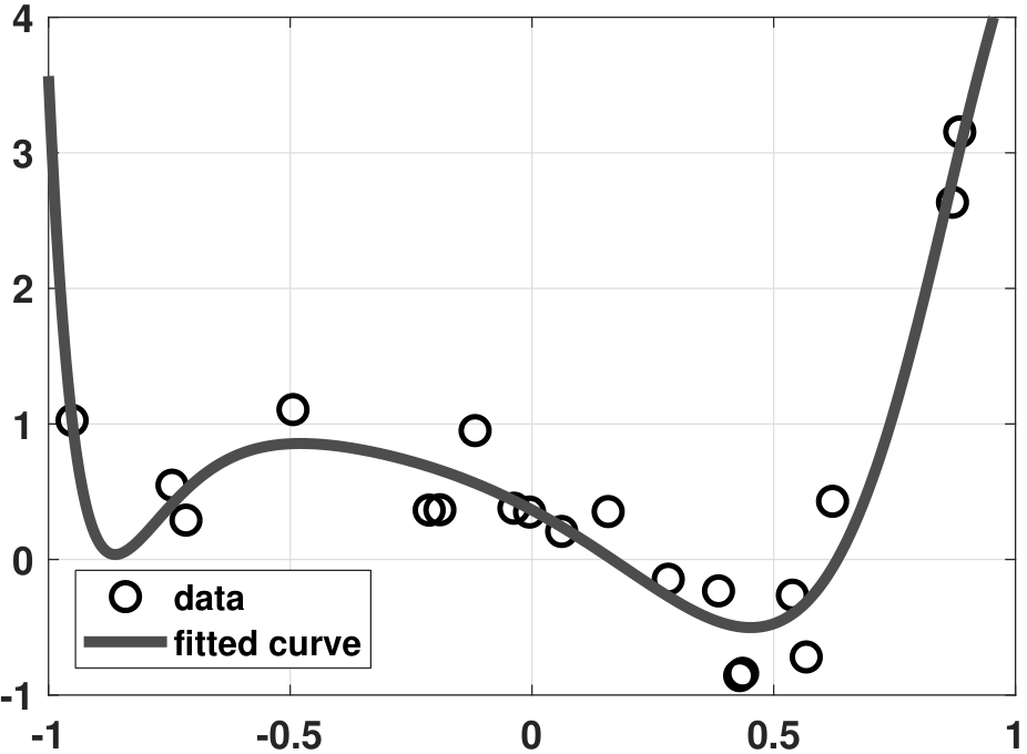
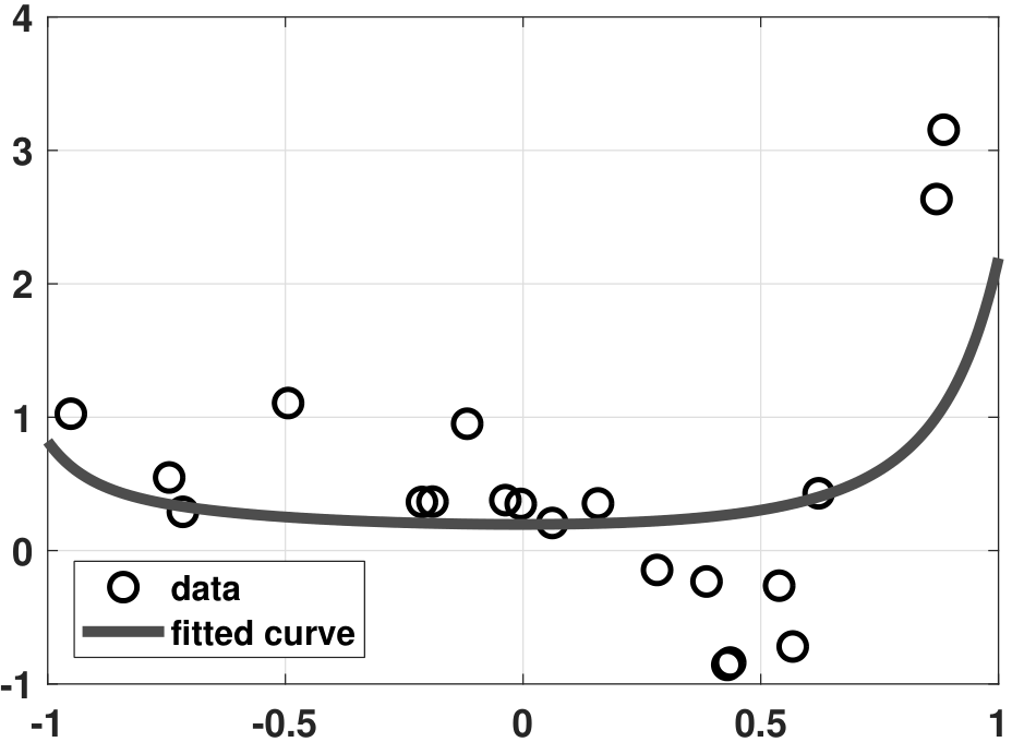
- (c) Next, we consider a ridge regression using three choices of \(\lambda\). The result is shown in Figure 7.17. If \(\lambda\) is too small, we observe that some overfitting still occurs. If \(\lambda\) is too large, then the curve underfits the data. For an appropriately chosen \(\lambda\), it can be seen that the fitting is reasonably good.
The MATLAB and Python codes used to generate the above plots are shown below.
% MATLAB code to demonstrate a ridge regression example
    % Generate data
    N = 20;
    x = linspace(-1,1,N);
    a = [0.5, -2, -3, 4, 6];
    y = a(1)+a(2)*x(:)+a(3)*x(:).^2+a(4)*x(:).^3+a(5)*x(:).^4+0.25*randn(N,1);

    % Ridge regression
    lambda = 0.1;
    d = 20;
    X = zeros(N, d);
    for p=0:d-1
        X(:,p+1) = x(:).^p;
    end
    A = [X; sqrt(lambda)*eye(d)];
    b = [y(:); zeros(d,1)];
    theta = A\b;

    % Interpolate and display results
    t    = linspace(-1, 1, 500);
    Xhat = zeros(length(t), d);
    for p=0:d-1
        Xhat(:,p+1) = t(:).^p;
    end
    yhat = Xhat*theta;
    plot(x,y,   'ko','LineWidth',2, 'MarkerSize', 10); hold on;
    plot(t,yhat,'LineWidth',4,'Color',[0.2 0.2 0.9]);
# Python code to demonstrate a ridge regression example
    import numpy as np
    import matplotlib.pyplot as plt
    from scipy.special import eval_legendre
    np.set_printoptions(precision=2, suppress=True)

    N = 20
    x = np.linspace(-1,1,N)
    a = np.array([0.5, -2, -3, 4, 6])
    y = a[0] + a[1]*x    + a[2]*x**2 + \
               a[3]*x**3 + a[4]*x**4 + 0.25*np.random.randn(N)
    d = 20
    X = np.zeros((N, d))
    for p in range(d):
      X[:,p] = x**p

    lambd = 0.1
    A = np.vstack((X, np.sqrt(lambd)*np.eye(d)))
    b = np.hstack((y, np.zeros(d)))
    theta = np.linalg.lstsq(A, b, rcond=None)[0]

    t    = np.linspace(-1, 1, 500)
    Xhat = np.zeros((500,d))
    for p in range(d):
      Xhat[:,p] = t**p
    yhat = np.dot(Xhat, theta)

    plt.plot(x,y,'o',markersize=12)
    plt.plot(t,yhat, linewidth=4)
plt.show()- sep0ex
The penalty term \(\|\vtheta\|^2\) in
$$\vthetahat_{\text{ridge}} = \argmin{\vtheta \in \R^d} \;\; \|\mX\vtheta - \vy\|^2 + \lambda\|\vtheta\|^2$$does not allow solutions with a very large \(\|\vtheta\|^2\).
- The penalty term adds a positive offset to the eigenvalues of \(\mX^T\mX\).
- Since the denominator in \((\mX^T\mX+\lambda\mI)^{-1}\mX^T\vy\) becomes larger than that of \((\mX^T\mX)^{-1}\mX^T\vy\), noise in \(\vy\) is less amplified.
Choosing the parameter
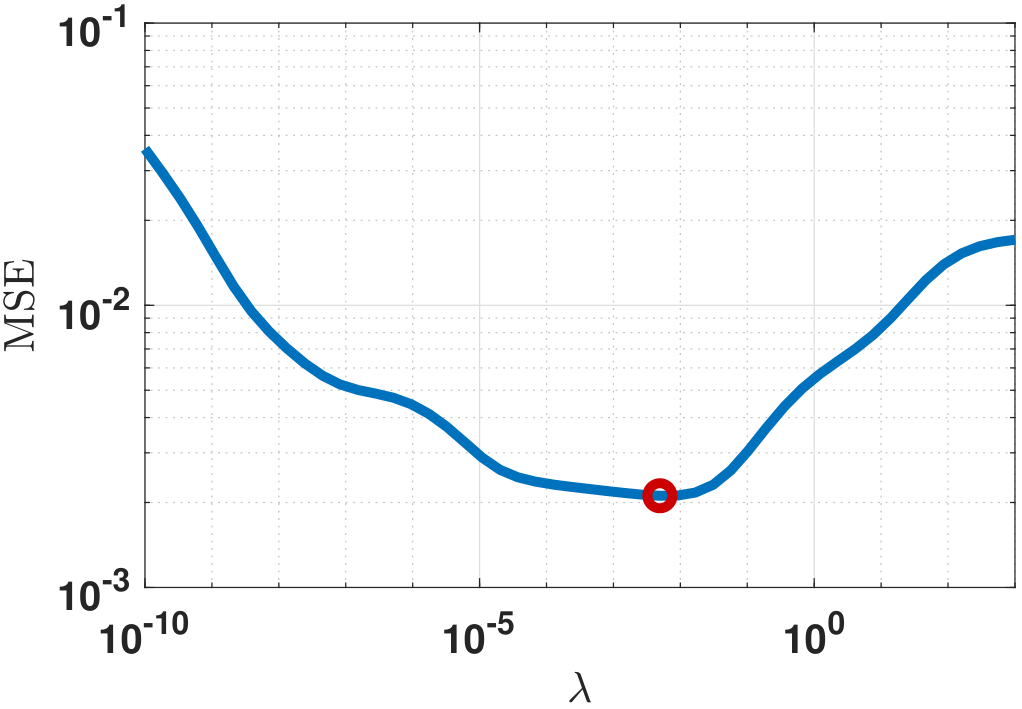
How should we choose the parameter \(\lambda\)? The honest answer is that there is no answer because the optimal \(\lambda\) can only be found if we have access to the testing samples. If we do, we can plot the MSE (the testing error) with respect to \(\lambda\), as shown in Figure 7.18(a).
Of course in reality we do not have access to the testing data. However, we can reserve a small portion of the training samples and treat them as validation samples. Then we run the ridge regression for different choices of \(\lambda\). The \(\lambda\) that minimizes the error on these validation samples is the one that you should deploy. If the training set is small, we can shuffle the validation samples randomly and compute the average. This scheme is known as cross-validation.
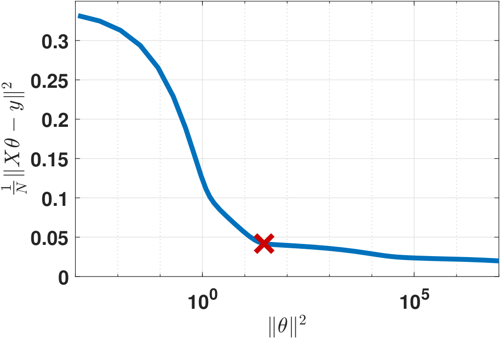
For some problems, there are “tactics” you may be able to employ for determining the optimal \(\lambda\). The first approach is to ask yourself what would be the reasonable range of \(\|\vtheta\|^2\) or \(\|\mX\vtheta-\vy\|^2\)? Are you expecting them to be large or small? Approximately in what order of magnitude? If you have some clues about this, then you can plot the function \(F(\vthetahat_{\lambda}) = \|\mX\vthetahat_{\lambda}-\vy\|^2\) as a function of \(R(\vthetahat_{\lambda}) = \|\vthetahat_{\lambda}\|^2\), where \(\vthetahat_{\lambda}\) is a shorthand notation for \(\vthetahat_{\text{ridge}}(\lambda)\), which is the estimated parameter using a specific value of \(\lambda\). Figure 7.18(b) shows an example of such a plot. As you can see, by varying \(\lambda\) we have different values of \(F(\vthetahat_{\lambda})\) and \(R(\vthetahat_{\lambda})\).
If you have some ideas about what \(\|\vtheta\|^2\) should be, say you want \(\|\vtheta\|^2 \le \tau\), you can go to the \(F(\vthetahat_{\lambda})\) versus \(R(\vthetahat_{\lambda})\) curve and find a point such that \(R(\vthetahat_{\lambda}) \le \tau\). On the other hand, if you want \(\|\mX\vtheta-\vy\|^2 \le \epsilon\), you can also go to the \(F(\vthetahat_{\lambda})\) versus \(R(\vthetahat_{\lambda})\) curve and find a point such that \(\|\mX\vtheta-\vy\|^2 \le \epsilon\). In either case, you have the freedom to shift the difficulty of finding \(\lambda\) to that of finding \(\tau\) or \(\epsilon\). Note that \(\tau\) and \(\epsilon\) have better physical interpretations. The quantity \(\epsilon\) tells us the upper bound of the prediction error, and \(\tau\) tells us the upper bound of the parameter magnitude. If you have been working on your dataset long enough, the historical data (and your experience) will help you determine these values.
Another feasible option suggested in the literature is finding the anchor point of the \(F(\vthetahat_{\lambda})\) and \(R(\vthetahat_{\lambda})\). The idea is that if the curve has a sharp elbow, the turning point would indicate a rapid increase/decrease in \(F(\vthetahat_{\lambda})\) (or \(R(\vthetahat_{\lambda})\)).
- sep0ex
- Cross-validation: Reserve a few training samples as validation samples. Check the prediction error w.r.t. these validation samples. The \(\lambda\) that minimizes the validation error is the one you deploy.
- \(\|\vtheta\|^2 \le \tau\): Plot the \(F(\vthetahat_{\lambda})\) and \(R(\vthetahat_{\lambda})\). Then go along the \(R\)-axis to find the position where \(R(\vthetahat_{\lambda}) \le \tau\).
- \(\|\mX\vtheta-\vy\|^2 \le \epsilon\): Plot the \(F(\vthetahat_{\lambda})\) and \(R(\vthetahat_{\lambda})\). Then go along the \(F\)-axis to find the position where \(F(\vthetahat_{\lambda}) \le \epsilon\).
- Find the elbow point of \(F(\vthetahat_{\lambda})\) and \(R(\vthetahat_{\lambda})\).
Bias and variance trade-off for ridge regression
We now discuss the bias and variance trade-off of the ridge regression.
Let \(\vy = \mX\vtheta+\ve\) be the training data, where \(\ve\) is zero-mean and has a covariance \(\sigma^2\mI\). Consider the ridge regression
Then the estimate has the properties that
where \(\mW_\lambda = (\mX^T\mX+\lambda\mI)^{-1}\mX^T\mX\).
Proof. The proof of this theorem involves some tedious matrix operations that will be omitted here. If you are interested in the proof you can consult van Wieringen's “Lecture notes on ridge regression”, https://arxiv.org/pdf/1509.09169.pdf.
■The results of this theorem provide a way to assess the bias and variance. Specifically, from the MSE we know that
The bias and variance are defined respectively as
We can then plot the bias and variance as a function of \(\lambda\). An example is shown in Figure 7.19.

The result in Figure 7.19 can be summarized in three points:
- sep0ex
- Bias \(\uparrow\) as \(\lambda \uparrow\). This is because a large \(\lambda\) pushes the solution towards \(\vtheta = 0\). Therefore, the bias with respect to the ground truth \(\vtheta\) will increase.
- Variance \(\downarrow\) as \(\lambda \uparrow\). Since variance is caused by noise, increasing \(\lambda\) forces the solution \(\vtheta\) to be small. Hence, it becomes less sensitive to noise.
- MSE reaches a minimum point somewhere in the middle. The MSE is the sum of bias and variance. Therefore, it drops to the minimum and then rises again as \(\lambda\) increases.
With appropriate choice of \(\lambda\), the ridge regression can have a lower mean squared error than the vanilla regression. The following result is due to C. M. Theobald: (Theobald, C. M. (1974). Generalizations of mean square error applied to ridge regression. Journal of the Royal Statistical Society. Series B (Methodological), 36(1), 103-106.)
For \(\lambda < 2\sigma^2\|\vtheta\|^{-2}\),
This theorem says that as long as \(\lambda\) is small enough, the ridge regression will have a lower MSE than the vanilla regression. Thus ridge regression is almost always helpful. Of course, the optimal \(\lambda\) is not provided by the theorem, which only tells us where to search for a good \(\lambda\).
- sep0ex
- The regularization reduces the variance (see Figure 7.19 when \(\lambda > 0\))
- It pays the price of increasing the bias.
- Usually, the drop in variance outweighs the increase in bias. So the overall MSE drops.
- Bias is not always a bad thing.
7.4.2LASSO regularization
The ridge regression we discussed in the previous subsection is just one of the many possible ways of doing regularization. One alternative is to replace \(\|\vtheta\|^2\) by \(\|\vtheta\|_1\), where
This change from the sum-squares to sum-absolute-values has been the main driving force in data science, machine learning, and signal processing for at least the past two decades. The optimization associated with \(\|\vtheta\|_1\) is
or
Seeking a sparse solution
To understand the choice of \(\|\cdot\|_1\), we need to introduce the concept of sparsity.
A vector \(\vtheta\) is called sparse if it has only a few non-zero elements.
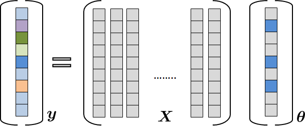
As illustrated in Figure 7.20, a sparse \(\vtheta\) ensures that only a very few columns of the data matrix \(\mX\) are active. This is an attractive property because, in some of the regression problems, it is indeed possible to have just a few dominant factors. The LASSO regression says that if our problem possesses this sparse solution, then the \(\|\cdot\|_1\) can help us find the sparse solution.
How can \(\|\vtheta\|_1\) promote sparsity? If we consider the sets
we note that \(\Omega_1\) has a diamond shape whereas \(\Omega_2\) has a circular shape. Since the data fidelity term \(\|\mX\vtheta-\vy\|^2\) is an ellipsoid, seeking the optimal value in the presence of the regularization term can be viewed as moving the ellipsoid until it touches the set defined by the regularization. As illustrated in Figure 7.21, since \(\{\vtheta \;|\; \|\vtheta\|^2 \le \tau \}\) is a circle, the solution will be somewhere in the middle. On the other hand, since \(\{\vtheta \;|\; \|\vtheta\|_1 \le \tau \}\) is a diamond, the solution will be one of the vertices. The difference between “somewhere in the middle” and “a vertex” is that the vertex is a sparse solution, since by the definition of a vertex one coordinate must be zero and the other coordinate must be non-zero. We can easily extrapolate this idea to the higher-dimensional spaces. In this case, we will see that the solution for the \(\|\cdot\|_1\) problem has only a few non-zero entries.

The optimization formulated in Eq. (7.41) is known as the least absolute shrinkage and selection operator (LASSO). LASSO problems are difficult, but over the past two decades we have increased our understanding of the problem. The most significant breakthrough is that we now have algorithms to solve the LASSO problem efficiently. This is important because, unlike the ridge regression, where we have a (very simple) closed-form solution, the LASSO problem can only be solved using iterative algorithms.
- sep0ex
- LASSO regularization promotes a sparse solution.
- If the underlying model has a sparse solution, e.g., you choose a 50th-order polynomial, but the underlying model is a third-order polynomial, then there should only be four non-zero regression coefficients in your 50th-order polynomial. LASSO will help in this case.
- If the underlying model has a dense solution, then LASSO is of limited value. A ridge regression could be better.
- While \(\|\vtheta\|_1\) is not differentiable (at 0), there exist polynomial-time convex algorithms to solve the problem, e.g., interior-point methods.
Solving the LASSO problem
Today, there are many open-source packages to solve the LASSO problem. They are mostly developed in the convex optimization literature. One of the most user-friendly packages is the CVX package developed by S. Boyd and colleagues at Stanford University. (The MATLAB version is here: http://cvxr.com/cvx/. The Python version is here: https://cvxopt.org/. Follow the instructions to install the package.) Once you have downloaded and installed the package, solving the optimization can be done literally by typing in the data fidelity term and the regularization term. An example is given below.
cvx_begin
        variable theta(d)
        minimize(sum_square(X*theta-y) + lambda*norm(theta,1))
    cvx_end
As you can see, the program is extremely simple. You start by calling cvx_begin and end it with cvx_end. Inside the box we create a variable theta(d), where d denotes the dimension of the vector theta. The main command is minimize. However, this line is almost self-explanatory. As long as you follow the syntax given by the user guidelines, you will be able to set it up properly.
In Python, we can call the cvxpy library.
import cvxpy as cvx
    theta     = cvx.Variable(d)
    objective = cvx.Minimize( cvx.sum_squares(X*theta-y) \
                                + lambd*cvx.norm1(theta) )
    prob      = cvx.Problem(objective)
    prob.solve()
To see a concrete example, we use the crime rate data obtained from https://web.stanford.edu/ hastie/StatLearnSparsity/data.html. A snapshot of the data is shown in the table below. In this dataset, the vector \(\vy\) is the crime rate, which is the last column of the table. The feature/basis vectors are funding, hs, not-hs, college.
| city | crime rate | funding | hs | no-hs | college |
| 1 | 478 | 40 | 74 | 11 | 31 |
| 2 | 494 | 32 | 72 | 11 | 43 |
| 3 | 643 | 57 | 71 | 18 | 16 |
| 4 | 341 | 31 | 71 | 11 | 25 |
| 50 | 940 | 66 | 67 | 26 | 18 |
We consider two optimizations:
As we have discussed, the first optimization uses the \(\|\cdot\|_1\) regularized least squares, which is the LASSO problem. The second optimization is the standard \(\|\cdot\|^2\) regularized least squares. Since both solutions depend on the parameter \(\lambda\), we parameterize the solutions in terms of \(\lambda\). Note that the optimal \(\lambda\) for \(\widehat{\vtheta}_{1}\) is not necessarily the optimal \(\lambda\) for \(\widehat{\vtheta}_{2}\).
One thing we would like to demonstrate in this example is visualizing the linear regression coefficients \(\widehat{\vtheta}_{1}(\lambda)\) and \(\widehat{\vtheta}_{2}(\lambda)\) as \(\lambda\) changes. To solve the optimization, we use CVX; the MATLAB and Python implementation is shown below.
data = load('./dataset/data_crime.txt');
    y    = data(:,1);        % The observed crime rate
    X    = data(:,3:end);    % Feature vectors
    [N,d]= size(X);

    lambdaset = logspace(-1,8,50);
    theta_store   = zeros(d,50);
    for i=1:length(lambdaset)
        lambda = lambdaset(i);
        cvx_begin
            variable theta(d)
            minimize( sum_square(X*theta-y) + lambda*norm(theta,1) )
    %       minimize( sum_square(X*theta-y) + lambda*sum_square(theta) )
        cvx_end
        theta_store(:,i) = theta(:);
    end

    figure(1);
    semilogx(lambdaset, theta_store, 'LineWidth', 4);
    legend('funding','% high', '% no high', '% college', ...
            '% graduate', 'Location','NW');
    xlabel('lambda');
ylabel('feature attribute');import cvxpy as cvx
import numpy as np
import matplotlib.pyplot as plt
data = np.loadtxt("/content/data_crime.txt")
y = data[:,0]
X = data[:,2:7]
N,d = X.shape
lambd_set = np.logspace(-1,8,50)
theta_store = np.zeros((d,50))
for i in range(50):
lambd = lambd_set[i]
theta = cvx.Variable(d)
objective = cvx.Minimize( cvx.sum_squares(X*theta-y) \
+ lambd*cvx.norm1(theta) )
# objective = cvx.Minimize( cvx.sum_squares(X*theta-y) \
+ lambd*cvx.sum_squares(theta) )
prob = cvx.Problem(objective)
prob.solve()
theta_store[:,i] = theta.value
for i in range(d):
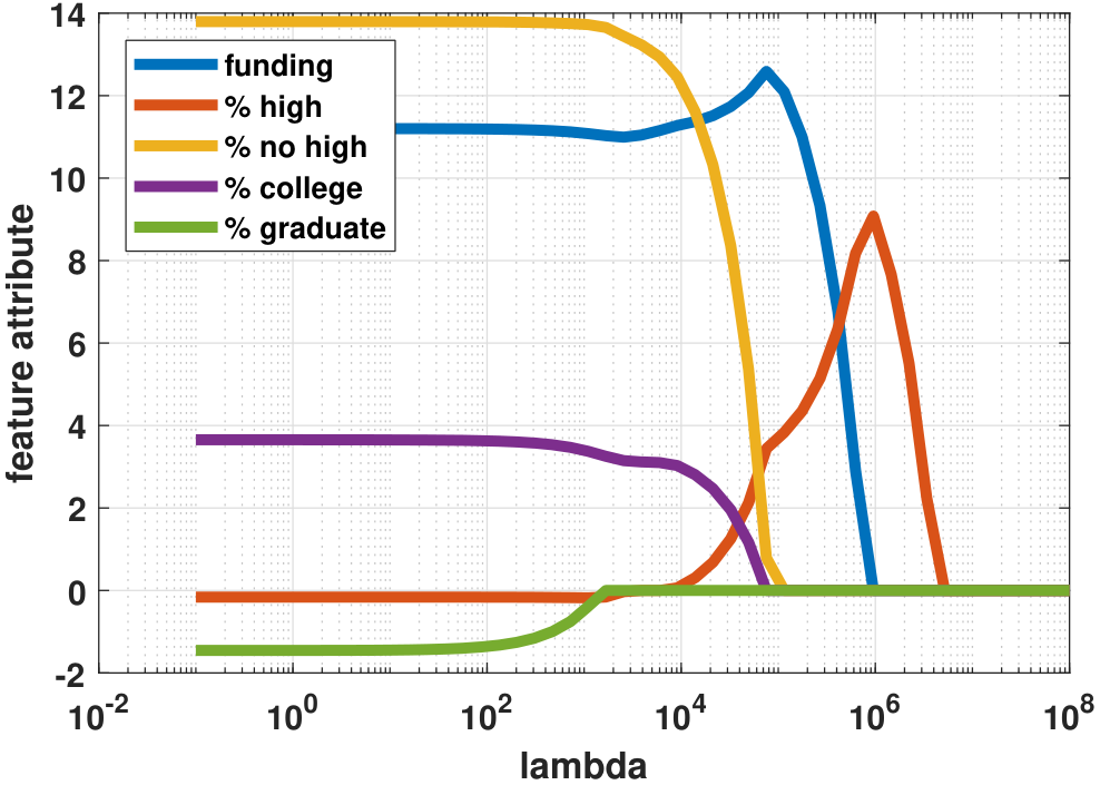
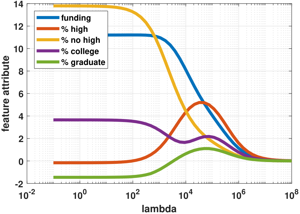
plt.semilogx(lambd_set, theta_store[i,:])Figure 7.22 shows some interesting differences between the two regression models.
- sep0ex
- Trajectory. For the \(\|\cdot\|^2\) estimate \(\vthetahat_2(\lambda)\), the trajectory of the regression coefficients is smooth. This is attributable to the fact that the training loss \(\calE_2(\vtheta)\) is continuously differentiable in \(\vtheta\), and so the solution trajectory is smooth. By contrast, the \(\|\cdot\|_1\) estimate \(\vthetahat_1(\lambda)\) has a more disruptive trajectory.
- Active members. For the LASSO problem, \(\vthetahat_1(\lambda)\) switches the active member as \(\lambda\) changes. For example, the feature
high-schoolis the first one being activated when \(\lambda \downarrow\). This implies that if we limit ourselves to only one feature, thenhigh-schoolis the feature we should select. The ridge regression does not have this feature-selection property. How about when \(\lambda = 10^6\)? In this case, the LASSO has two active members:fundingandhigh-school. This suggests that if there are two contributing factors,fundingandhigh-schoolare the two. When \(\lambda = 10^4\), we see that in LASSO, the green curve goes to zero but then the red curve rises. This means a correlation betweenhigh schoolandno high school, which should not be a surprise because they are complementary to each other. - Magnitude of solutions. The magnitude of the solutions does not necessarily convey a clear conclusion because the feature vectors (e.g.,
high school) and the observablecrime ratehave different units. - Limiting solutions. As \(\lambda \rightarrow 0\), both \(\vthetahat_1(\lambda)\) and \(\vthetahat_2(\lambda)\) reach the same solution, because the training losses are identical when \(\lambda = 0\).
LASSO for overfitting
Does LASSO help to mitigate the overfitting problem? Not always, but it often does. In Figure 7.23 we consider fitting a dataset of \(N=20\) data points. The ground truth model we use is
where \(e_n \sim \text{Gaussian}(0,\sigma^2)\) for \(\sigma = 0.25\). When fitting the data, we purposely choose a 20th-order Legendre polynomial as the regression model. With only \(N=20\) data points, we can be almost certain that there is overfitting.
The MATLAB and Python codes for solving this LASSO problem are shown below.
% MATLAB code to demonstrate overfitting and LASSO
    % Generate data
    N = 20;
    x = linspace(-1,1,N)';
    a = [1, 0.5, 0.5, 1.5, 1];
    y = a(1)*legendreP(0,x)+a(2)*legendreP(1,x)+a(3)*legendreP(2,x)+ ...
        a(4)*legendreP(3,x)+a(5)*legendreP(4,x)+0.25*randn(N,1);

    % Solve LASSO using CVX
    d = 20;
    X = zeros(N, d);
    for p=0:d-1
        X(:,p+1) = reshape(legendreP(p,x),N,1);
    end
    lambda = 2;
    cvx_begin
        variable theta(d)
        minimize( sum_square( X*theta - y ) + lambda * norm(theta , 1) )
    cvx_end

    % Plot results
    t    = linspace(-1, 1, 200);
    Xhat = zeros(length(t), d);
    for p=0:d-1
        Xhat(:,p+1) = reshape(legendreP(p,t),200,1);
    end
    yhat = Xhat*theta;
    plot(x,y,   'ko','LineWidth',2, 'MarkerSize', 10); hold on;
    plot(t,yhat,'LineWidth',6,'Color',[0.2 0.5 0.2]);
# Python code to demonstrate overfitting and LASSO
    import cvxpy as cvx
    import numpy as np
    import matplotlib.pyplot as plt

    # Setup the problem
    N = 20
    x = np.linspace(-1,1,N)
    a = np.array([1, 0.5, 0.5, 1.5, 1])
    y = a[0]*eval_legendre(0,x) + a[1]*eval_legendre(1,x) + \
        a[2]*eval_legendre(2,x) + a[3]*eval_legendre(3,x) + \
        a[4]*eval_legendre(4,x) + 0.25*np.random.randn(N)

    # Solve LASSO using CVX
    d = 20
    lambd = 1
    X = np.zeros((N, d))
    for p in range(d):
      X[:,p] = eval_legendre(p,x)
    theta       = cvx.Variable(d)
    objective   = cvx.Minimize( cvx.sum_squares(X*theta-y) \
                                + lambd*cvx.norm1(theta) )
    prob        = cvx.Problem(objective)
    prob.solve()
    thetahat = theta.value

    # Plot the curves
    t = np.linspace(-1, 1, 500)
    Xhat = np.zeros((500,d))
    for p in range(P):
      Xhat[:,p] = eval_legendre(p,t)
    yhat = np.dot(Xhat, thetahat)
    plt.plot(x, y, 'o')
    plt.plot(t, yhat, linewidth=4)
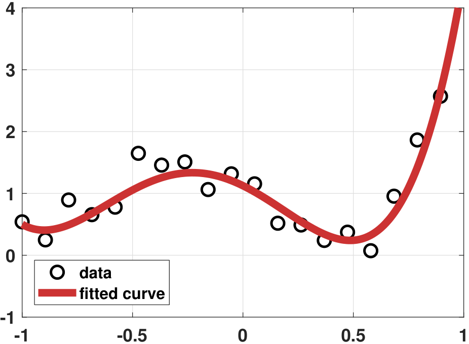
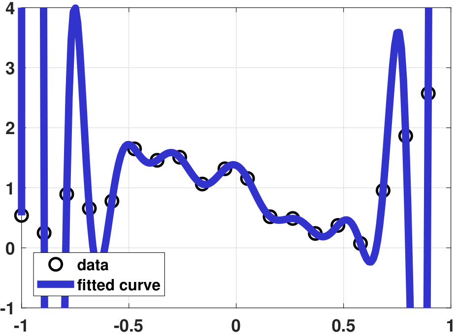
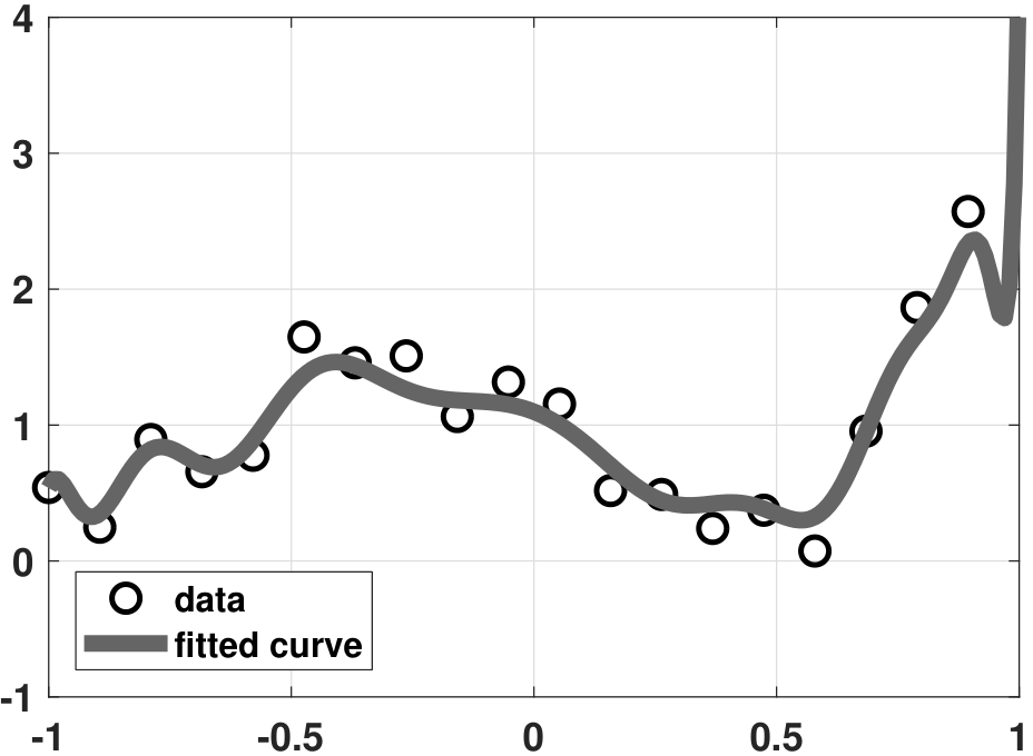
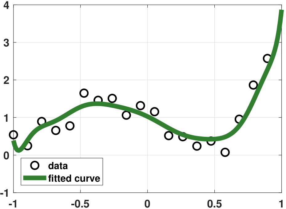
Let us compare the various regression results. Figure 7.23(b) shows the vanilla regression, which as you can see fits the \(N = 20\) data points very well. However, no one would believe that such a fitting curve can generalize to unseen data. Figure 7.23(c) shows the ridge regression result. When performing the analysis, we sweep a range of \(\lambda\) and pick the value \(\lambda = 0.5\) so that the fitted curve is neither too “wild” nor too “flat”. We can see that the fitting is improved. However, since the ridge regression only penalizes large-magnitude coefficients, the fitting is still not ideal. Figure 7.23(d) shows the LASSO regression result. Since the true model is a 4th-order polynomial and we use a 20th-order polynomial, the true solution is sparse. Therefore, LASSO is helpful, and hence we can pick a sparse solution.
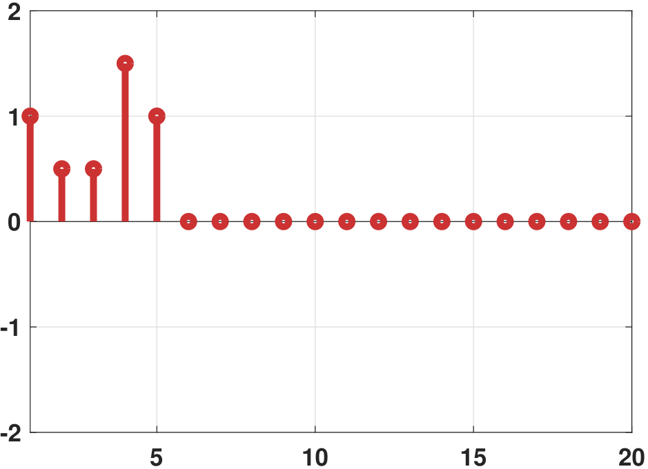
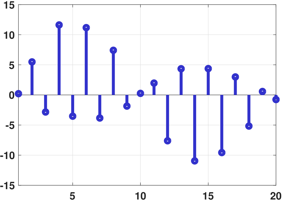
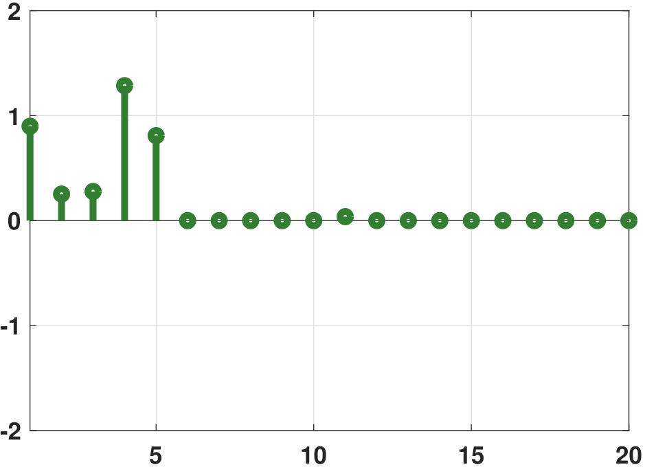
The significance of LASSO is often not about the fitting of the data points but the number of active coefficients. In Figure 7.24 we show a comparison between the ground truth coefficients, the vanilla regression coefficients, the ridge regression coefficients, and the LASSO regression coefficients. It is evident that the LASSO solution contains a much smaller number of non-zeros compared to the ridge regression. Most of the high-order coefficients are zero. By contrast, the vanilla regression coefficients are wild. The ridge regression is better, but there are many non-zero high-order coefficients.

Closing remark. In this section, we discussed two regularization techniques: ridge regression and LASSO regression. Both techniques are about adding a penalty term to the training loss to constrain the regression coefficients. In the optimization literature, writings on ridge and LASSO regression are abundant, covering both algorithms and theoretical properties. An example of a theoretical question addressed in the literature is: Under what conditions is LASSO guaranteed to recover the correct support of the solution, i.e., locating the correct positions of the non-zeros? Problems like these are beyond the scope of this book.