Bias and Variance Trade-Off

Our linear analysis has provided you with a rough understanding of what we experience in overfitting. However, for general regression problems where the models are not necessarily linear, we need to go deeper. The goal of this section is to explain the trade-off between bias and variance. This analysis requires some patience as it involves many equations. We recommend skipping this section on a first reading and then returning to it later.

7.3.1Decomposing the testing error

Notations

As we did at the beginning of Section 7.2, we consider a ground truth model that relates an input \(\vx\) and an output \(y\):

where \(e \sim \text{Gaussian}(0,\sigma^2)\) is the noise. For example, if we use a linear model, then \(f\) could be \(f(\vx) = \vtheta^T\vx\), for some regression coefficients \(\vtheta\).

During training, we pick a prediction model \(g_{\vtheta}(\cdot)\) and try to predict the output when given a training sample \(\vx\):

For example, we may choose \(g_{\vtheta}(\vx) = \vtheta^T\vx\), which is also a linear model. We may also choose a linear model in another basis, e.g., \(g_{\vtheta}(\vx) = \vtheta^T\phi(\vx)\) for some transformations \(\phi(\cdot)\). In any case, the goal of training is to minimize the training error:

where the sum is taken over the training samples \(\calD_{\text{train}} = \{(\vx_1,y_1),\ldots,(\vx_N,y_N)\}\). Because the model parameter \(\vthetahat\) is learned from the training dataset \(\calD_{\text{train}}\), the prediction model depends on \(\calD_{\text{train}}\). To emphasize this dependency, we write

During testing, we consider a testing dataset \(\calD_{\text{test}} = \{(\vx_1',y_1'),\ldots,(\vx_M',y_M')\}\). We put these testing samples into the trained model to predict an output:

Since the goal of regression is to make \(g^{(\calD_{\text{train}})}\) as close to \(f\) as possible, it is natural to expect \(\yhat_m'\) to be close to \(y_m'\).

Testing error decomposition (noise-free)

So we can now compute the testing error — the error that we ultimately care about. In the noise-free condition, i.e., \(e = 0\), the testing error is defined as

There are several components in this equation. First, \(\vx'\) is a testing sample drawn from a certain distribution. You can think of \(\calD_{\text{test}}\) as a finite subset drawn from this distribution. Second, the error \(\big(g^{(\calD_{\text{train}})}(\vx') - f(\vx') \big)^2\) measures the deviation between our predicted value and the true value. Note that this error term is specific to one testing sample \(\vx'\). Therefore, we take expectation \(\E_{\vx'}\) to find the average of the error for the distribution of \(\vx'\).

The testing error \(\calE_{\text{test}}^{(\calD_{\text{train}})}\) is a function that is dependent on the training set \(\calD_{\text{train}}\), because the model \(g^{(\calD_{\text{train}})}\) is trained from \(\calD_{\text{train}}\). Therefore, as we change the training set, we will have a different model \(g\) and hence a different testing error. To eliminate the randomness of the training set, we define the overall testing error as

Note that this definition of the testing error is consistent with the special case in Eq. (7.20), in which the testing error involves a joint expectation over \(\ve\) and \(\ve'\). The expectation over \(\ve\) accounts for the training samples, and the expectation over \(\ve'\) accounts for the testing samples.

Let us try to extract some meaning from the testing error. Our method will be to decompose the testing error into bias and variance.

Let's consider what this theorem implies. This result is a decomposition of the testing error into bias and variance. It is a universal result that applies to all regression models, not only linear cases. To summarize the meanings of bias and variance:

Figure 7.11 gives a pictorial representation of bias and variance. In this figure, we construct four scenarios of bias and variance. Each cross represents the predictor \(g^{(\calD_{\text{train}})}\), with the true predictor \(f\) at the origin. Figure 7.11(a) shows the case with a low bias and a low variance. All of these predictors \(g^{(\calD_{\text{train}})}\) are very close to the ground truth, and they have small fluctuations around their average. Figure 7.11(b) shows the case of a high bias and a low variance. It has a high bias because the entire group of \(g^{(\calD_{\text{train}})}\) is shifted to the corner. The bias, which is the distance from the truth to the average, is therefore large. The variance remains small because the fluctuation around the average is small. Figure 7.11(c) shows the case of a low bias but high variance. In this case, the fluctuation around the average is large. Figure 7.11(d) shows the case of high bias and high variance. We want to avoid this case.

Testing error decomposition (noisy case)

Let us consider a situation when there is noise. In the presence of noise, the training and testing samples will follow the relationship

where \(e \sim \text{Gaussian}(0,\sigma^2)\). We assume that the noise is Gaussian to make the proof easier. We can consider other types of noise in theory, but the theoretical results will need to be modified.

In the presence of noise, the testing error is

where we take the joint expectation over the training dataset \(\calD_{\text{train}}\) and the error \(e\). Continuing the calculation, and using the fact that \(\calD_{\text{train}}\) and \(e\) are independent (and \(\E[e] = 0\)), it follows that

Taking the expectation of \(\vx'\) over the entire testing distribution gives us

The theorem below summarizes the results:

7.3.2Analysis of the bias

Let us examine the bias and variance in more detail. To discuss bias we must first understand the quantity

which is known as the average predictor. The average predictor, as the equation suggests, is the expectation of the predictor \(g^{(\calD_{\text{train}})}\). Remember that \(g^{(\calD_{\text{train}})}\) is a predictor constructed from a specific training set \(\calD_{\text{train}}\). If tomorrow our training set \(\calD_{\text{train}}\) contains other data (that come from the same underlying distribution), \(g^{(\calD_{\text{train}})}\) will be different. The average predictor \(\overline{g}\) is the average across these random fluctuations of the dataset \(\calD_{\text{train}}\). Here is an example:

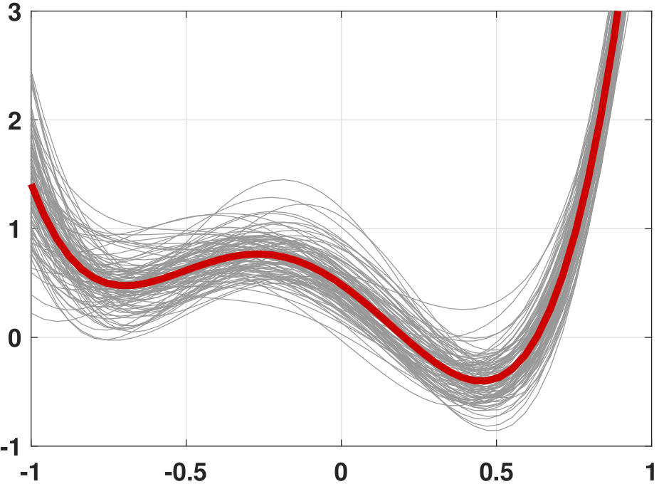
Suppose we use a linear model with the ordinary polynomials as the bases. The data points are generated according to

If we use a particular training set \(\calD_{\text{train}}\) and run the regression, we will be able to obtain one of the regression lines, as shown in Figure 7.12. Let us call this line \(g^{(1)}\). We repeat the experiment by drawing another dataset, and call it \(g^{(2)}\). We continue and eventually we will find a set of regression lines \(g^{(1)}, g^{(2)}, \ldots, g^{(K)}\), where \(K\) denotes the number of training sets you are using to generate all the gray curves. The average predictor \(\overline{g}\) is defined as

Thus if we take the average of all of these gray curves we will obtain the average predictor, which is the red curve shown in Figure 7.12.

If you are curious about how this plot was generated, the MATLAB and Python codes are given below.

% MATLAB code to visualize the average predictor
    N = 20;
    a = [5.7, 3.7, -3.6, -2.3, 0.05];
    x = linspace(-1,1,N);
    yhat = zeros(100,50);
    for i=1:100
        X    = [x(:).^0, x(:).^1, x(:).^2, x(:).^3, x(:).^4];
        y    = X*a(:) + 0.5*randn(N,1);
        theta = X\y(:);
        t    = linspace(-1, 1, 50);
        yhat(i,:) = theta(1) + theta(2)*t(:)   + theta(3)*t(:).^2 ...
                             + theta(4)*t(:)^3 + theta(5)*t(:).^4;
    end
    figure;
    plot(t, yhat, 'color', [0.6 0.6 0.6]); hold on;
    plot(t, mean(yhat), 'LineWidth', 4, 'color', [0.8 0 0]);
    axis([-1 1 -2 2]);

import numpy as np
    import matplotlib.pyplot as plt
    from scipy.special import eval_legendre
    np.set_printoptions(precision=2, suppress=True)
    
    N = 20
    x = np.linspace(-1,1,N)
    a = np.array([0.5, -2, -3, 4, 6])
    yhat = np.zeros((50,100))
    for i in range(100):
      y = a[0] + a[1]*x    + a[2]*x**2 + \
                 a[3]*x**3 + a[4]*x**4 + 0.5*np.random.randn(N)
      X = np.column_stack((np.ones(N), x, x**2, x**3, x**4))
    
      theta = np.linalg.lstsq(X, y, rcond=None)[0]
      t = np.linspace(-1,1,50)
      Xhat = np.column_stack((np.ones(50), t, t**2, t**3, t**4))
      yhat[:,i] = np.dot(Xhat, theta)
      plt.plot(t, yhat[:,i], c='gray')
    plt.plot(t, np.mean(yhat, axis=1), c='r', linewidth=4)

We now show an analytic calculation to verify Figure 7.12.

In the above example, we obtained an interesting result, namely that \(\overline{g}(\vx') = f(\vx')\). That is, the average predictor equals the true predictor. However, in general, \(\overline{g}(\vx')\) does not necessarily equal \(f(\vx')\). If this occurs, we have a deviation \((\overline{g}(\vx')-f(\vx'))^2 > 0\). This deviation is called the bias. Bias is independent of the number of training samples because we have taken the average of the predictors. Therefore, bias is more of an intrinsic (or systematic) error due to the choice of the model.

7.3.3Variance

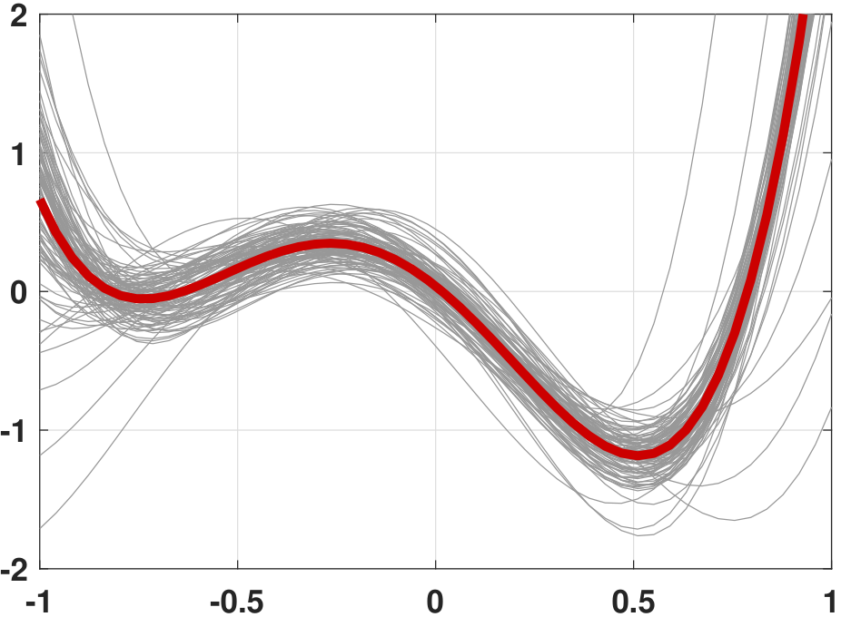
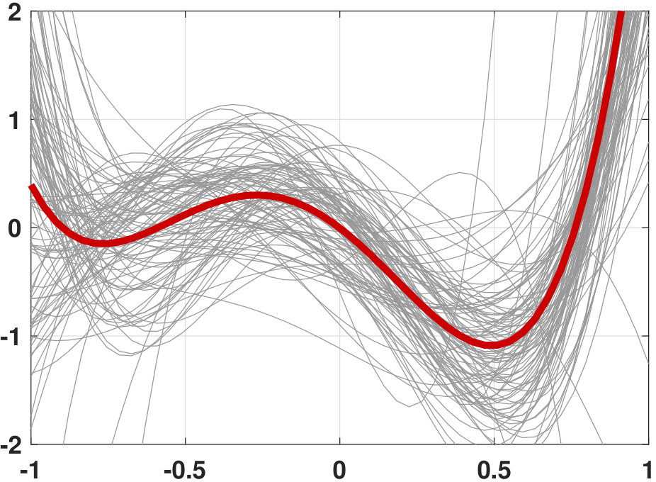
The other quantity in the game is the variance. Variance at a testing sample \(\vx'\) is defined as

As the equation suggests, the variance measures the fluctuation between the predictor \(g^{(\calD_{\text{train}})}\) and the average predictor \(\overline{g}\). Figure 7.13 illustrates the polynomial-fitting problem we discussed above. In this figure we consider two levels of variance by varying the noise strength of \(e_n\). The figure shows that as the observation becomes noisier, the predictor \(g^{(\calD_{\text{train}})}\) will have a larger fluctuation around the average predictor.

What will happen if we use more samples so that \(N\) grows? As \(N\) grows, the matrix \(\mX\) will have more rows. Assuming that the magnitude of the entries remains unchanged, more rows in \(\mX\) will increase the magnitude of \(\mX^T\mX\) because we are summing more terms. Consider a \(2 \times 2\) ordinary polynomial system where

As \(N\) grows, all the entries in the matrix grow. As a result, \((\mX^T\mX)^{-1}\) will shrink in magnitude and thus drive the variance \(\sigma^2 \text{Tr}\Big\{ (\mX^T\mX)^{-1} (\vx')(\vx')^T \Big\}\) to zero.

7.3.4Bias and variance on the learning curve

The decomposition of the testing error into bias and variance is portrayed visually by the learning curve shown in Figure 7.14. This figure shows the testing error and the training error as functions of the number of training samples. As \(N\) increases, we observe that both testing and training errors converge to the same value. At any fixed \(N\), the testing error is composed of bias and variance:

• sep0ex
• The bias is the distance from the ground truth to the steady-state level. This value is fixed and is a constant w.r.t. \(N\). In other words, regardless of how many training samples you have, the bias is always there. It is the best outcome you can achieve.
• The variance is the fluctuation from the steady-state level to the instantaneous state. It drops as \(N\) increases.

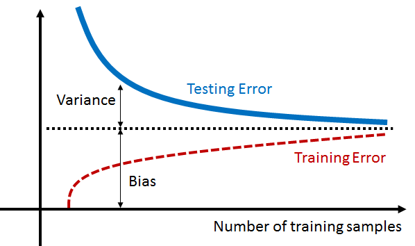
Figure 7.15 compares the learning curve of two models. The first case requires us to fit the data using a simple model (marked in purple). The training error and the testing error have small fluctuations around the steady-state because, for simple models, you need only a small number of samples to make the model happy. The second case requires us to fit the data using a complex model (marked in green). This set of curves has a much wider fluctuation because it is harder to train and harder to generalize. However, when we have enough training samples, the training error and the testing error will converge to a lower steady-state value. Therefore, you need to pay the price of using a complex model, but if you do, you will enjoy a lower testing error.

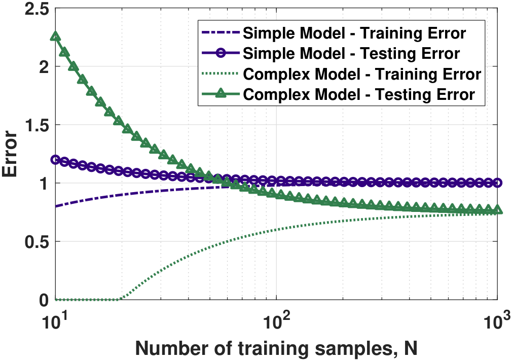
The implication of all this is that you should choose the model by considering the number of data points. Never buy an expensive toy when you do not have the money! If you insist on using a complex model while you do not have enough training data, you will suffer from a poor testing error even if you feel good about it.

Closing remark. We close this section by revisiting the bias-variance trade-off:

The relationship among the three terms is summarized below: