eBook › Chapter 8 · Estimation

Section 8.2

Properties of ML Estimates

ML estimation is a very special type of estimation. Not all estimations are ML. If an estimate is ML, are there any theoretical properties we can analyze? For example, will ML estimates guarantee the recovery of the true parameter? If so, when will this happen? In this section we investigate these theoretical questions so that you will acquire a better understanding of the statistical nature of ML estimates. (For notational simplicity, in this section we will focus on a scalar parameter $\theta$ instead of a vector parameter $\vtheta$. )

8.2.1Estimators

We know that an ML estimate is defined as

\thetahat_{\text{ML}}(\vx) = \argmax{\theta} \;\; \calL(\theta \,|\, \vx).

We write $\thetahat_{\text{ML}}(\vx)$ to emphasize that $\thetahat_{\text{ML}}$ is a function of $\vx$. The dependency of $\thetahat_{\text{ML}}(\vx)$ on $\vx$ should not be a surprise. For example, if the ML estimate is the sample average, we have that

\thetahat_{\text{ML}}(x_1,\ldots,x_N) = \frac{1}{N} \sum_{n=1}^N x_n,

where $\vx = [x_1,\ldots,x_N]^T$.

However, in this setting we should always remember that $x_1,\ldots,x_N$ are realizations of the i.i.d. random variables $X_1,\ldots,X_N$. Therefore, if we want to analyze the randomness of the variables, it is more reasonable to write $\thetahat_{\text{ML}}$ as a random variable $\widehat{\Theta}_{\text{ML}}$. For example, in the case of sample average, we have that

\widehat{\Theta}_{\text{ML}}(X_1,\ldots,X_N) = \frac{1}{N} \sum_{n=1}^N X_n.

We call $\widehat{\Theta}_{\text{ML}}$ the ML estimator of the true parameter $\theta.$

Estimate versus estimator

sep0ex
An estimate is a number, e.g., $\displaystyle \thetahat_{\text{ML}} = \frac{1}{N} \sum_{n=1}^N x_n$. It is the random realization of a random variable.
An estimator is a random variable, e.g., $\displaystyle \widehat{\Theta}_{\text{ML}} = \frac{1}{N} \sum_{n=1}^N X_n$. It takes a set of random variables and generates another random variable.

The ML estimators are one type of estimator, namely those that maximize the likelihood functions. If we do not want to maximize the likelihood we can still define an estimator. An estimator is any function that takes the data points $X_1,\ldots,X_N$ and maps them to a number (or a vector of numbers). That is, an estimator is

\widehat{\Theta}(X_1,\ldots,X_N).

We call $\widehat{\Theta}$ the estimator of the true parameter $\theta$.

Example 8.11

Let $X_1,\ldots,X_N$ be Gaussian i.i.d. random variables with unknown mean $\theta$ and known variance $\sigma^2$. Construct two possible estimators.

Solution

We define two estimators:

\begin{aligned} \widehat{\Theta}_1(X_1,\ldots,X_N) &= \frac{1}{N}\sum_{n=1}^N X_n,\\ \widehat{\Theta}_2(X_1,\ldots,X_N) &= X_1, \end{aligned}

In the first case, the estimator takes all the samples and constructs the sample average. The second estimator takes all the samples and returns only the first element. Both are legitimate estimators. However, $\widehat{\Theta}_1$ is the ML estimator, whereas $\widehat{\Theta}_2$ is not.

8.2.2Unbiased estimators

While you can define estimators in any way you like, certain estimators are good and others are bad. By “good” we mean that the estimator can provide you with the information about the true parameter $\theta$; otherwise, why would you even construct such an estimator? However, the difficulty here is that $\widehat{\Theta}$ is a random variable because it is constructed from $X_1,\ldots,X_N$. Therefore, we need to define different metrics to quantify the usefulness of the estimators.

Definition 8.5

An estimator $\widehat{\Theta}$ is unbiased if

\E[\widehat{\Theta}] = \theta.

Unbiasedness means that the average of the random variable $\widehat{\Theta}$ matches the true parameter $\theta$. In other words, while we allow $\widehat{\Theta}$ to fluctuate, we expect the average to match the true $\theta$. If this is not the case, using more measurements will not help us get closer to $\theta$.

Example 8.12

Let $X_1,\ldots,X_N$ be i.i.d. Gaussian random variables with an unknown mean $\theta$. It has been shown that the ML estimator is

\widehat{\Theta}_{\text{ML}} = \frac{1}{N}\sum_{n=1}^{N} X_n.

Is the ML estimator $\widehat{\Theta}_{\text{ML}}$ unbiased?

Solution

To check the unbiasedness, we look at the expectation:

\begin{aligned} \E[\widehat{\Theta}_{\text{ML}}] &= \frac{1}{N}\sum_{n=1}^{N} \E[X_n] = \frac{1}{N}\sum_{n=1}^{N} \theta = \theta. \end{aligned}

Thus, $\widehat{\Theta}_{\text{ML}} = \frac{1}{N} \sum_{n=1}^N X_n$ is an unbiased estimator of $\theta$.

Example 8.13

Same as the example before, but this time we consider an estimator

\widehat{\Theta} = X_1+X_2+5.

Is this estimator unbiased?

Solution

In this case,

\begin{aligned} \E[\widehat{\Theta}] &= \E[X_1+X_2+5] = \E[X_1] + \E[X_2] + 5 = 2\theta+5 \not= \theta. \end{aligned}

Therefore, the estimator is biased.

Example 8.14

Let $X_1,\ldots,X_N$ be i.i.d. Gaussian random variables with unknown mean $\mu$ and unknown variance $\sigma^2$. We have shown that the ML estimators are

\begin{aligned} \widehat{\mu}_{\text{ML}} = \frac{1}{N}\sum_{n=1}^N X_n \qquad\mbox{and}\qquad \widehat{\sigma}^2_{\text{ML}} = \frac{1}{N} \sum_{n=1}^N (X_n-\widehat{\mu}_{\text{ML}})^2. \end{aligned}

It is easy to show that $\E[\widehat{\mu}_{\text{ML}}] = \mu$. How about $\widehat{\sigma}^2_{\text{ML}}$? Is it an unbiased estimator?

Solution

For simplicity we assume $\mu = 0$ so that $\E[X_n^2] = \E[(X_n-0)^2] = \sigma^2$.

Note that

\begin{aligned} \E[\widehat{\sigma}^2_{\text{ML}}] &= \frac{1}{N}\sum_{n=1}^N \bigg\{\E[X_n^2] - 2\E[\muhat_{\text{ML}} X_n] + \E[\muhat_{\text{ML}}^2]\bigg\}\\ &= \frac{1}{N} \sum_{n=1}^N \left\{ \sigma^2 - 2\E\left[ \frac{1}{N}\sum_{j=1}^N X_j X_n\right] + \E\left[\left(\frac{1}{N}\sum_{n=1}^N X_n\right)^2\right] \right\}. \end{aligned}

By independence, we observe that $\E[X_jX_n] = \E[X_j]\E[X_n] = 0$, for any $j \not= n$. Therefore,

\begin{aligned} \E\left[ \frac{1}{N}\sum_{j=1}^N X_j X_n\right] &= \frac{1}{N}\E\bigg[X_1X_n + \cdots + X_N X_n\bigg]\\ &= \frac{1}{N}(0 + \cdots + \sigma^2 + \cdots + 0)=\frac{\sigma^2}{N}. \end{aligned}

Similarly, we have that

\begin{aligned} \E\left[\left(\frac{1}{N}\sum_{n=1}^N X_n\right)^2\right] &= \frac{1}{N^2}\sum_{n=1}^N \left\{\E[X_n^2] + \sum_{j\not=n} \E[X_jX_n]\right\}\\ &= \frac{1}{N^2}\sum_{n=1}^N \Big\{\sigma^2 + 0\Big\}= \frac{\sigma^2}{N}. \end{aligned}

Combining everything, we arrive at the result:

\begin{aligned} \E[\widehat{\sigma}^2_{\text{ML}}] &= \frac{1}{N} \sum_{n=1}^N \left\{ \sigma^2 - 2\E\left[ \frac{1}{N}\sum_{j=1}^N X_j X_n\right] + \E\left[\left(\frac{1}{N}\sum_{n=1}^N X_n\right)^2\right] \right\}\\ &= \frac{1}{N} \sum_{n=1}^N \left\{ \sigma^2 - \frac{2\sigma^2}{N} + \frac{\sigma^2}{N} \right\} \\ &= \frac{N-1}{N}\sigma^2, \end{aligned}

which is not equal to $\sigma^2$. Therefore, $\widehat{\sigma}^2_{\text{ML}}$ is a biased estimator of $\sigma^2$.

In the previous example, it is possible to construct an unbiased estimator for the variance. To do so, we can use

\widehat{\sigma}^2_{\text{unbias}} = \frac{1}{N-1}\sum_{n=1}^N (X_n-\widehat{\mu}_{\text{ML}})^2,

so that $\E[\widehat{\sigma}^2_{\text{unbias}}] = \sigma^2$. However, note that $\widehat{\sigma}^2_{\text{unbias}}$ does not maximize the likelihood, so while you can get unbiasedness, you cannot maximize the likelihood. If you want to maximize the likelihood, you cannot get unbiasedness.

What is an unbiased estimator?

sep0ex
An estimator $\widehat{\Theta}$ is unbiased if $\E[\widehat{\Theta}] = \theta$.
Unbiased means that the statistical average of $\widehat{\Theta}$ is the true parameter $\theta$.
If $X_n \sim \text{Gaussian}(\theta,\sigma^2)$, then $\widehat{\Theta} = (1/N)\sum_{n=1}^N X_n$ is unbiased and consistent, but $\widehat{\Theta} = X_1$ is unbiased but inconsistent.

8.2.3Consistent estimators

By definition, an estimator $\Thetahat(X_1,\ldots,X_N)$ is a function of $N$ random variables $X_1,\ldots,X_N$. Therefore, $\Thetahat(X_1,\ldots,X_N)$ changes as $N$ grows. In this subsection we analyze how $\Thetahat$ behaves when $N$ changes. For notational simplicity we use the following notation:

\Thetahat_N = \Thetahat(X_1,\ldots,X_N).

Thus, as $N$ increases, we use more random variables in defining $\Thetahat(X_1,\ldots,X_N)$.

Definition 8.6

An estimator $\Thetahat_N$ is consistent if $\Thetahat_N \overset{p}{\longrightarrow} \theta$, i.e.,

\lim_{N\rightarrow \infty} \Pb\bigg[\left|\Thetahat_N - \theta\right| \ge \epsilon\bigg] = 0.

The definition here follows from our discussions of the law of large numbers in Chapter 6. The specific type of convergence is known as the convergence in probability. It says that as $N$ grows, the estimator $\Thetahat$ will be close enough to $\theta$ so that the probability of getting a large deviation will diminish, as illustrated in Figure 8.11.

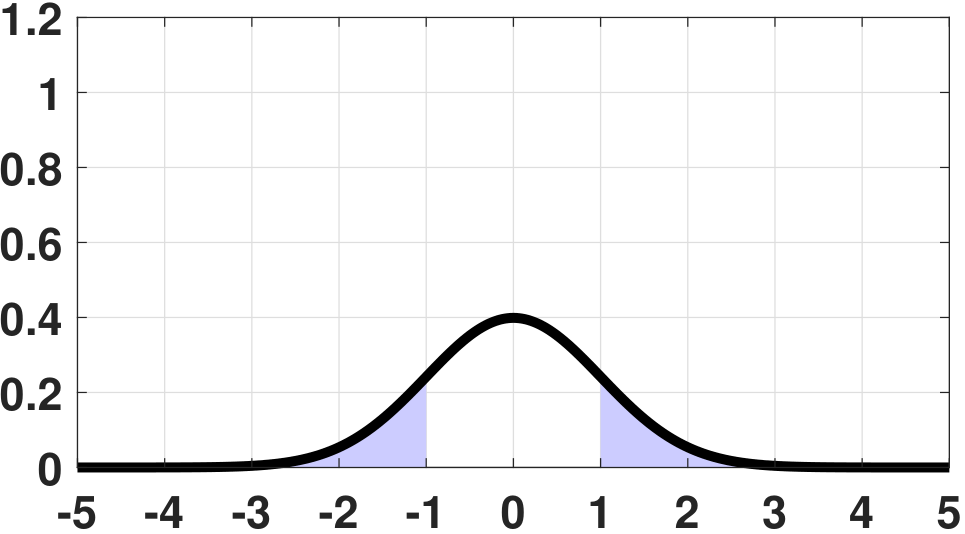
**Figure 8.11.** The four subfigures here illustrate the probability of error $\Pb\big[|\Thetahat_N - \theta| \ge \epsilon\big]$, which is represented by the areas shaded in blue. We assume that the estimator $\Thetahat_N$ is a Gaussian random variable following a distribution $\text{Gaussian}(0,\frac{\sigma^2}{N})$, where we set $\sigma = 1$. The threshold we use in this figure is $\epsilon = 1$. As $N$ grows, we see that the probability of error diminishes. If the probability of error goes to zero, we say that the estimator is consistent.

The examples in Figure 8.11 are typical situations using the sample average. For example, if we assume that $X_1,\ldots,X_N$ are i.i.d. Gaussian copies of $\text{Gaussian}(0,\sigma^2)$, then the estimator

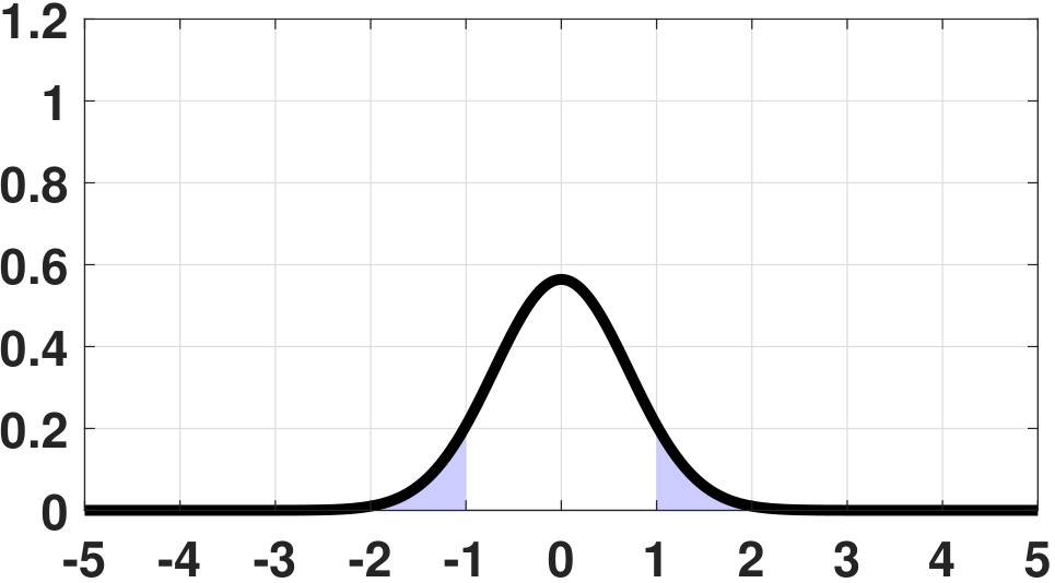
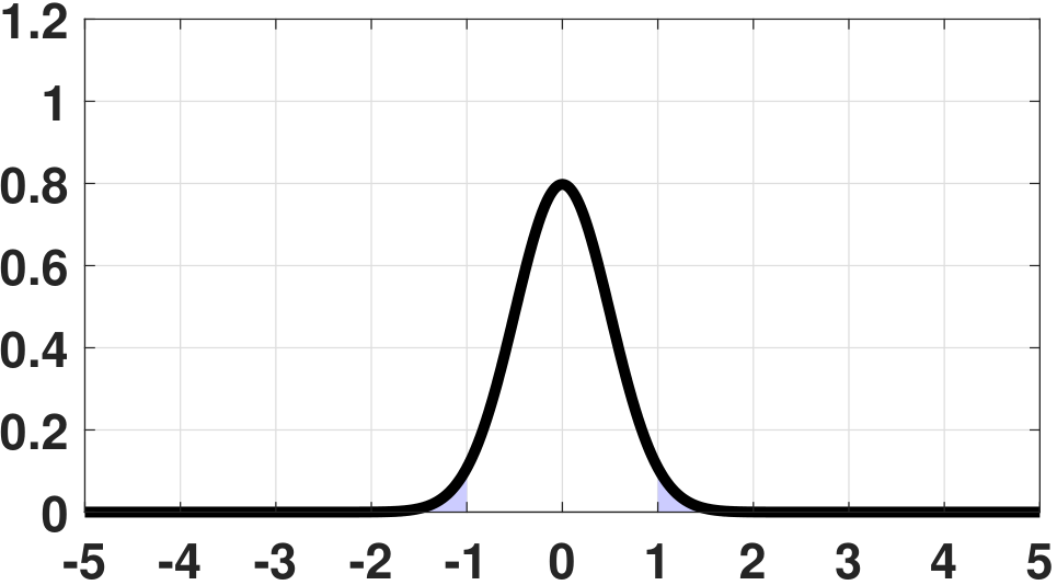
\Thetahat(X_1,\ldots,X_N) = \frac{1}{N}\sum_{n=1}^N X_n

will follow a Gaussian distribution $\text{Gaussian}(0,\frac{\sigma^2}{N})$. (Please refer to Chapter 6 for the derivation.) Then, as $N$ grows, the PDF of $\Thetahat_N$ becomes narrower and narrower. For a fixed $\epsilon$, it follows that the probability of error will diminish to zero. In fact, we can prove that, for this example,

\begin{aligned} \Pb\bigg[\left|\Thetahat_N - \theta\right| \ge \epsilon\bigg] &= \Pb\bigg[\Thetahat_N - \theta \ge \epsilon\bigg] + \Pb\bigg[\Thetahat_N - \theta \le -\epsilon\bigg]\\ &= \int_{\theta+\epsilon}^{\infty} \text{Gaussian}\left(z\,\big|\,\theta,\frac{\sigma^2}{N}\right) \;dz + \int_{-\infty}^{\theta-\epsilon} \text{Gaussian}\left(z\,\big|\,\theta,\frac{\sigma^2}{N}\right) \;dz\\ &= \int_{\theta+\epsilon}^{\infty} \frac{1}{\sqrt{2\pi \sigma^2/N}}e^{-\frac{(z-\theta)^2}{2\sigma^2/N}} \;dz + \int_{-\infty}^{\theta-\epsilon} \frac{1}{\sqrt{2\pi \sigma^2/N}}e^{-\frac{(z-\theta)^2}{2\sigma^2/N}} \;dz\\ &= \int_{\frac{\epsilon}{\sigma/\sqrt{N}}}^{\infty} \frac{1}{\sqrt{2\pi}}e^{-\frac{z^2}{2}} \;dz + \int_{-\infty}^{-\frac{\epsilon}{\sigma/\sqrt{N}}} \frac{1}{\sqrt{2\pi}}e^{-\frac{z^2}{2}} \;dz\\ &= 1-\Phi\left(\frac{\epsilon}{\sigma/\sqrt{N}}\right) + \Phi\left(\frac{-\epsilon}{\sigma/\sqrt{N}}\right)\\ &= 2\Phi\left(\frac{-\epsilon}{\sigma/\sqrt{N}}\right). \end{aligned}

Therefore, as $N \rightarrow \infty$, it holds that $\frac{-\epsilon}{\sigma/\sqrt{N}} \rightarrow -\infty$. Hence,

\lim_{N\rightarrow\infty} \Pb\bigg[\left|\Thetahat_N - \theta\right| \ge \epsilon\bigg] = \lim_{N\rightarrow\infty} 2\Phi\left(\frac{-\epsilon}{\sigma/\sqrt{N}}\right) = 0.

This explains why in Figure 8.11 the probability of error diminishes to zero as $N$ grows. Therefore, we say that $\Thetahat_N$ is consistent.

In general, there are two ways to check whether an estimator is consistent:

sep0ex
Prove convergence in probability. This is based on the definition of a consistent estimator. If we can prove that
$\lim_{N\rightarrow \infty} \Pb\big[|\Thetahat_N - \theta| \ge \epsilon\big] = 0,$
then we say that the estimator is consistent.
Prove convergence in mean squared error:
$\lim_{N\rightarrow \infty}\E[(\Thetahat_N - \theta)^2] = 0.$
To see why convergence in the mean squared error is sufficient to guarantee consistency, we recall Chebyshev's inequality in Chapter 6, which says that
$\begin{aligned} \Pb\big[|\Thetahat_N - \theta| \ge \epsilon\big] \le \frac{\E[(\Thetahat_N - \theta)^2]}{\epsilon^2}. \end{aligned}$
Thus, if $\lim_{N\rightarrow \infty}\E[(\Thetahat_N - \theta)^2] = 0$, convergence in probability will also hold. However, since mean square convergence is stronger than convergence in probability, being unable to show mean square convergence does not imply that an estimator is inconsistent.

Be careful not to confuse a consistent estimator with an unbiased estimator. The two are different concepts; one does not imply the other.

Consistent versus unbiased

sep0ex
Consistent = If you have enough samples, then the estimator $\widehat{\Theta}$ will converge to the true parameter.
Unbiasedness does not imply consistency. For example (Gaussian), if $$\widehat{\Theta} = X_1,$$ then $\E[X_1] = \mu$. But $\Pb[|\Thetahat-\mu|>\epsilon]$ does not converge to 0 as $N$ grows. So this estimator is inconsistent. (See Example 8.16 below.)
Consistency does not imply unbiasedness. For example (Gaussian), $$\widehat{\Theta} = \frac{1}{N}\sum_{n=1}^N (X_n-\mu)^2$$ is a biased estimate for variance, but it is consistent. (See Example 8.17 below.)

Example 8.15

Let $X_1,\ldots,X_N$ be i.i.d. Gaussian random variables with an unknown mean $\mu$ and known variance $\sigma^2$. We know that the ML estimator for the mean is $\widehat{\mu}_{\text{ML}} = (1/N)\sum_{n=1}^N X_n$. Is $\widehat{\mu}_{\text{ML}}$ consistent?

Solution

We have shown that the ML estimator is

\begin{aligned} \widehat{\mu}_{\text{ML}} = \frac{1}{N}\sum_{n=1}^N X_n. \end{aligned}

Since $\E[\widehat{\mu}_{\text{ML}}] = \mu$, and $\E[(\widehat{\mu}_{\text{ML}}-\mu)^2] = \Var[\widehat{\mu}_{\text{ML}}] = \frac{\sigma^2}{N}$, it follows that

\Pb\big[|\widehat{\mu}_{\text{ML}} - \mu| \ge \epsilon\big] \le \frac{\E[(\widehat{\mu}_{\text{ML}} - \mu)^2]}{\epsilon^2} = \frac{\sigma^2}{N\epsilon^2}.

Thus, when $N$ goes to infinity, the probability converges to zero, and hence the estimator is consistent.

Example 8.16

Let $X_1,\ldots,X_N$ be i.i.d. Gaussian random variables with an unknown mean $\mu$ and known variance $\sigma^2$. Define an estimator $\muhat = X_1$. Show that the estimator is unbiased but inconsistent.

Solution

We know that $\E[\muhat] = \E[X_1] = \mu$. So $\muhat$ is an unbiased estimator. However, we can show that $$\E[(\muhat-\mu)^2] = \E[(X_1-\mu)^2] = \sigma^2.$$ Since this variance $\E[(\muhat-\mu)^2]$ does not shrink as $N$ increases, it follows that no matter how many samples we use we cannot make $\E[(\muhat-\mu)^2]$ go to zero. To be more precise,

\begin{aligned} \Pb\bigg[\left|\widehat{\mu} - \mu\right| \ge \epsilon\bigg] &= \Pb\bigg[\left|X_1 - \mu\right| \ge \epsilon\bigg] \\ &= \Pb\bigg[X_1 \le \mu - \epsilon\bigg] + \Pb\bigg[X_1 \ge \mu + \epsilon\bigg]\\ &= \int_{-\infty}^{\mu-\epsilon} \frac{1}{\sqrt{2\pi\sigma^2}}e^{-\frac{(x-\mu)^2}{2\sigma^2}} \;dx + \int_{\mu+\epsilon}^{\infty} \frac{1}{\sqrt{2\pi\sigma^2}}e^{-\frac{(x-\mu)^2}{2\sigma^2}} \;dx \\ &= 2\Phi\left(\frac{-\epsilon}{\sigma}\right), \end{aligned}

which does not converge to zero as $N \rightarrow \infty$. So the estimator is inconsistent.

Example 8.17

Let $X_1,\ldots,X_N$ be i.i.d. Gaussian random variables with an unknown mean $\mu$ and an unknown variance $\sigma^2$. Is the ML estimate of the variance, i.e., $\sigmahat_{\text{ML}}^2$, consistent?

Solution

We know that the ML estimator for the mean is

\muhat_{\text{ML}} = \frac{1}{N}\sum_{n=1}^N X_n,

and we have shown that it is an unbiased and consistent estimator of the mean. For the variance,

\begin{aligned} \sigmahat_{\text{ML}}^2 = \frac{1}{N}\sum_{n=1}^N \left(X_n - \muhat_{\text{ML}}\right)^2 &= \frac{1}{N}\sum_{n=1}^N \left[X_n^2 - 2\muhat_{\text{ML}} X_n + \muhat_{\text{ML}}^2 \right]\\ &= \frac{1}{N}\sum_{n=1}^N X_n^2 - 2 \muhat_{\text{ML}} \cdot \frac{1}{N}\sum_{n=1}^N X_n + \muhat_{\text{ML}}^2\\ &= \frac{1}{N}\sum_{n=1}^N X_n^2 - \muhat_{\text{ML}}^2. \end{aligned}

Note that $\frac{1}{N}\sum_{n=1}^N X_n^2$ is the sample average of the second moment, and so by the weak law of large numbers it should converge in probability to $\E[X_n^2]$. Similarly, $\muhat_{\text{ML}}$ will converge in probability to $\mu$. Therefore, we have

\begin{aligned} \sigmahat_{\text{ML}}^2 = \frac{1}{N}\sum_{n=1}^N X_n^2 - \muhat_{\text{ML}}^2 &\overset{p}{\longrightarrow} (\sigma^2 + \mu^2) - \mu^2 = \sigma^2. \end{aligned}

Thus, we have shown that the ML estimator of the variance is biased but consistent.

The following discussions about the consistency of ML estimators can be skipped.

As we have said, there are many estimators. Some estimators are consistent and some are not. The ML estimators are special. It turns out that under certain regularity conditions the ML estimators of i.i.d. observations are consistent.

Without proving this result formally, we highlight a few steps to illustrate the idea. Suppose that we have a set of i.i.d. data points $\vx_1,\ldots,\vx_N$ drawn from some distribution $f(\vx ;\, \vtheta_{\text{true}})$. To formulate the ML estimation, we consider the log-likelihood function (divided by $N$):

\frac{1}{N} \log \calL(\vtheta \,|\, \vx) = \frac{1}{N} \sum_{n=1}^N \log f(\vx_n;\,\vtheta).

Here, the variable $\vtheta$ is unknown. We need to find it by maximizing the log-likelihood.

By the weak law of large numbers, we can show that the log-likelihood based on the $N$ samples will converge in probability to

\begin{aligned} \underset{g_N(\vtheta)}{\underbrace{\frac{1}{N} \sum_{n=1}^N \log f(\vx_n;\,\vtheta)} } \overset{p}{\longrightarrow} \E[\log f(\vx;\,\vtheta)]. \end{aligned}

The expectation can be evaluated by integrating over the true distribution:

\E[\log f(\vx;\,\vtheta)] = \underset{g(\vtheta)}{ \underbrace{\int \log f(\vx;\,\vtheta) \cdot f(\vx;\,\vtheta_{\text{true}}) d\vx}}.

where $f(\vx;\,\vtheta_{\text{true}})$ denotes the true distribution of the samples $\vx_n$'s. From these two results we define two functions:

\begin{aligned} g_N(\vtheta) \bydef \frac{1}{N} \sum_{n=1}^N \log f(\vx_n;\,\vtheta), \;\; \mbox{and} \;\; g(\vtheta) \bydef \int \log f(\vx;\,\vtheta) \cdot f(\vx;\,\vtheta_{\text{true}}) d\vx, \end{aligned}

and we know that $g_N(\vtheta) \overset{p}{\longrightarrow} g(\vtheta)$.

We also know that $\vthetahat_{\text{ML}}$ is the ML estimator, and so

\vthetahat_{\text{ML}} = \argmax{\vtheta} \;\; g_N(\vtheta).

Let $\vtheta^*$ be the maximizer of the limiting function, i.e.,

\vtheta^* = \argmax{\vtheta} \;\; g(\vtheta).

Because $g_N(\vtheta) \overset{p}{\rightarrow} g(\vtheta)$, we can (loosely (To rigorously prove this statement we need some kind of regularity conditions on $g_N$ and $g$. A more formal proof can be found in H. Vincent Poor, An Introduction to Signal Detection and Estimation, Springer, 1998, Section IV.D.)) argue that $\vthetahat_{\text{ML}} \overset{p}{\rightarrow} \vtheta^*$. If we can show that $\vtheta^* = \vtheta_{\text{true}}$, then we have shown that $\vthetahat_{\text{ML}} \overset{p}{\rightarrow} \vtheta_{\text{true}}$, implying that $\vthetahat_{\text{ML}}$ is consistent.

To show that $\vtheta^* = \vtheta_{\text{true}}$, we note that

\begin{aligned} \frac{d}{d\vtheta} \; \int \log f(\vx;\,\vtheta) \cdot f(\vx;\,\vtheta_{\text{true}})\, d\vx &= \int \frac{d}{d\vtheta} \log f(\vx;\,\vtheta) \cdot f(\vx;\,\vtheta_{\text{true}})\, d\vx\\ &= \int \frac{f'(\vx;\,\vtheta)}{f(\vx;\,\vtheta)} \cdot f(\vx;\,\vtheta_{\text{true}})\, d\vx. \end{aligned}

We ask whether this is equal to zero. Putting $\vtheta = \vtheta_{\text{true}}$, we have that

\begin{aligned} \int \frac{f'(\vx;\,\vtheta_{\text{true}})}{f(\vx;\,\vtheta_{\text{true}})} \cdot f(\vx;\,\vtheta_{\text{true}})\, d\vx = \int f'(\vx;\;\vtheta_{\text{true}})\, d\vx. \end{aligned}

However, this integral can be simplified to

\begin{aligned} \int f'(\vx;\;\vtheta_{\text{true}})\, d\vx &= \frac{d}{d\vtheta} \underset{=1}{\underbrace{\int f(\vx;\;\vtheta)\, d\vx}} \bigg|_{\vtheta = \vtheta_{\text{true}}} = 0. \end{aligned}

Therefore, $\vtheta_{\text{true}}$ is the maximizer for $g(\vtheta)$, and so $\vtheta_{\text{true}} = \vtheta^*$.

End of the discussion. Please join us again.

8.2.4Invariance principle

Another useful property satisfied by the ML estimate is the invariance principle. The invariance principle says that a monotonic transformation of the true parameter is preserved for the ML estimates.

What is the invariance principle?

sep0ex
There is a monotonic function $h$.
There is an ML estimate $\widehat{\theta}_{\text{ML}}$ for $\theta$.
The monotonic function $h$ maps the true parameter $\theta \longmapsto h(\theta)$.
Then the same function will map the ML estimate $\widehat{\theta}_{\text{ML}} \longmapsto h(\widehat{\theta}_{\text{ML}})$.

The formal statement of the invariance principle is given by the theorem below.

Theorem 8.1

If $\widehat{\theta}_{\text{ML}}$ is the ML estimate of $\theta$, then for any one-to-one function $h$ of $\theta$, the ML estimate of $h(\theta)$ is $h(\widehat{\theta}_{\text{ML}})$.

Proof. Define the likelihood function $\calL(\theta)$ (we have dropped $\vx$ to simplify the notation). Then, for any monotonic function $h$, we have that

\begin{aligned} \calL(\theta) = \calL(h^{-1}(h(\theta))). \end{aligned}

Let $\thetahat_{\text{ML}}$ be the ML estimate:

\begin{aligned} \thetahat_{\text{ML}} &= \argmax{\theta} \; \calL(\theta) = \argmax{\theta} \; \calL(h^{-1}(h(\theta))). \end{aligned}

By the definition of ML, $\thetahat_{\text{ML}}$ must maximize the likelihood. Therefore, $\calL(h^{-1}(h(\theta)))$ is maximized when $h^{-1}(h(\theta)) = \thetahat_{\text{ML}}$. This implies that $h(\theta) = h(\thetahat_{\text{ML}})$ because $h$ is monotonic. Since $h(\theta)$ is the parameter we try to estimate, the equality $h(\theta) = h(\thetahat_{\text{ML}})$ implies that $h(\thetahat_{\text{ML}})$ is the ML estimate of $h(\theta)$.

■

Example 8.18

Consider the single-photon image sensor example we discussed in Section 8.1. We consider a set of i.i.d. Bernoulli random variables with PMF

p_{X_n}(1) = 1-e^{-\eta} \qquad \text{and} \qquad p_{X_n}(0) = e^{-\eta}.

Find the ML estimate through (a) direct calculation and (b) the invariance principle.

Solution

(a) Following the example in Eq. (8.12), the ML estimate of $\eta$ is

\begin{aligned} \widehat{\eta}_{\text{ML}} &= \argmax{\eta}\; \prod_{n=1}^N (1-e^{-\eta})^{x_n}(e^{-\eta})^{1-x_n} \\ &= -\log\left(1-\frac{1}{N}\sum_{n=1}^N x_n\right). \end{aligned}

(b) We can obtain the same result using the invariance principle. Since $X_n$ is a binary random variable, we assume that it is a Bernoulli with parameter $\theta$. Then the ML estimate of $\theta$ is

\begin{aligned} \widehat{\theta}_{\text{ML}} &= \argmax{\theta} \prod_{n=1}^N \theta^{x_n}(1-\theta)^{1-x_n} \\ &= \frac{1}{N}\sum_{n=1}^N x_n. \end{aligned}

The relationship between $\theta$ and $\eta$ is that $\theta = 1-e^{-\eta}$, or $\eta = -\log(1-\theta)$. So we let $h(\theta) = -\log(1-\theta)$. The invariance principle says that the ML estimate of $h(\theta)$ is

\begin{aligned} \widehat{\eta}_{\text{ML}} &\bydef \widehat{h(\theta)}_{\text{ML}}\\ &\overset{(i)}{=} h(\widehat{\theta}_{\text{ML}}) \\ &= -\log\left(1-\frac{1}{N}\sum_{n=1}^N x_n\right), \end{aligned}

where (i) follows from the invariance principle.

The invariance principle can be very convenient, especially when the transformation $h$ is complicated, so that a direct evaluation of the ML estimate is difficult.

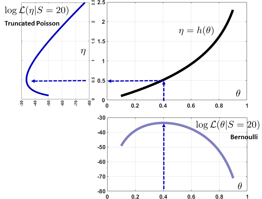
The invariance principle is portrayed in Figure 8.12. We start with the Bernoulli log-likelihood

\begin{aligned} \log\calL(\theta|S) = S\log\theta + (N-S)\log(1-\theta). \end{aligned}

In this particular example we let $S = 20$, where $S$ denotes the sum of the $N = 50$ Bernoulli random variables. The other log-likelihood is the truncated Poisson, which is given by

\begin{aligned} \log\calL(\eta|S) = S\log(1-e^{-\eta}) + (N-S)\log(e^{-\eta}). \end{aligned}

The transformation between the two is the function

\eta = h(\theta) = -\log(1-\theta).

Putting everything into the figure, we see that the ML estimate ($\theta = 0.4$) is translated to $\eta = 0.5108$. The invariance principle asserts that this calculation can be done by $\widehat{\eta}_{\text{ML}} = h(\widehat{\theta}_{\text{ML}}) = h(0.4) = 0.5108$.