Maximum A Posteriori Estimation
In ML estimation, the parameter \(\vtheta\) is treated as a deterministic quantity. There are, however, many situations where we have some prior knowledge about \(\vtheta\). For example, we may not know exactly the speed of a car, but we may know that the speed is roughly 65 mph with a standard deviation of 5 mph. How do we incorporate such prior knowledge into the estimation problem?
In this section, we introduce the second estimation technique, known as the maximum a posteriori (MAP) estimation. MAP estimation links the likelihood and the prior. The key idea is to treat the parameter \(\vtheta\) as a random variable (vector) \(\mTheta\) with a PDF \(f_{\mTheta}(\vtheta)\).
8.3.1The trio of likelihood, prior, and posterior
To understand how the MAP estimation works, it is important first to understand the role of the parameter \(\vtheta\), which changes from a deterministic quantity to a random quantity.
Recall the likelihood function we defined in the ML estimation; it is
if we assume that we have a set of i.i.d. observations \(\vx = [x_1,\ldots,x_N]^T\). By writing the PDF of \(\mX\) as \(f_{\mX}(\vx; \, \vtheta)\), we emphasize that \(\vtheta\) is a deterministic but unknown parameter. There is nothing random about \(\vtheta\).
In MAP, we change the nature of \(\vtheta\) from deterministic to random. We replace \(\vtheta\) by \(\mTheta\) and write
The difference between the left-hand side and the right-hand side is subtle but important. On the left-hand side, \(f_{\mX}(\vx; \, \vtheta)\) is the PDF of \(\mX\). This PDF is parameterized by \(\vtheta\). On the right-hand side, \(f_{\mX|\mTheta}(\vx | \vtheta)\) is a conditional PDF of \(\mX\) given \(\mTheta\). The values they provide are exactly the same. However, in \(f_{\mX|\mTheta}(\vx | \vtheta)\), \(\vtheta\) is a realization of a random variable \(\mTheta\).
Because \(\mTheta\) is now a random variable (vector), we can define its PDF (yes, the PDF of \(\mTheta\)), and denote it by
which is called the prior distribution. The prior distribution of \(\mTheta\) is unique in MAP estimation. There is nothing called a prior in ML estimation.
Multiplying \(f_{\mX|\mTheta}(\vx | \vtheta)\) with the prior PDF \(f_{\mTheta}(\vtheta)\), and using Bayes' theorem, we obtain the posterior distribution:
The posterior distribution is the PDF of \(\mTheta\) given the measurements \(\mX\).
The likelihood, the prior, and the posterior can be confusing. Let us clarify their meanings.
- sep0ex
- Likelihood \(f_{\mX|\mTheta}(\vx|\vtheta)\): This is the conditional probability density of \(\mX\) given the parameter \(\mTheta\). Do not confuse the likelihood \(f_{\mX|\mTheta}(\vx|\vtheta)\) defined in the MAP context with the likelihood \(f_{\mX}(\vx; \vtheta)\) defined in the ML context. The former assumes that \(\mTheta\) is random whereas the latter assumes that \(\vtheta\) is deterministic. They have the same values.
- Prior \(f_{\mTheta}(\vtheta)\): This is the prior distribution of \(\mTheta\). It does not come from the data \(\mX\) but from our prior knowledge. For example, if we see a bike on the road, even before we take any measurement we will have a rough idea of its speed. This is the prior distribution.
- Posterior \(f_{\mTheta|\mX}(\vtheta|\vx)\): This is the posterior density of \(\mTheta\) given that we have observed \(\mX\). Do not confuse \(f_{\mTheta|\mX}(\vtheta|\vx)\) with \(\calL(\vtheta \,|\, \vx)\). The posterior distribution \(f_{\mTheta|\mX}(\vtheta|\vx)\) is a PDF of \(\mTheta\) given \(\mX = \vx\). The likelihood \(\calL(\vtheta \,|\, \vx)\) is not a PDF. If you integrate \(f_{\mTheta|\mX}(\vtheta|\vx)\) with respect to \(\vtheta\), you get 1, but if you integrate \(\calL(\vtheta \,|\, \vx)\) with respect to \(\vtheta\), you do not get 1.
| Likelihood | ML | \(f_{\mX}(\vx; \; \vtheta)\) The parameter \(\vtheta\) is deterministic. |
| MAP | \(f_{\mX|\mTheta}(\vx \;|\; \vtheta)\) The parameter \(\mTheta\) is random. | |
| Prior | ML | There is no prior, because \(\vtheta\) is deterministic. |
| MAP | \(f_{\mTheta}(\vtheta)\) This is the PDF of \(\mTheta\). | |
| Optimization | ML | Find the peak of the likelihood \(f_{\mX}(\vx; \; \vtheta)\). |
| MAP | Find the peak of the posterior \(f_{\mTheta|\mX}(\vtheta \;|\; \vx)\). | |
Maximum a posteriori (MAP) estimation is a form of Bayesian estimation. Bayesian methods emphasize our prior knowledge or beliefs about the parameters. As we will see shortly, the prior has something valuable to offer, especially when we have very few data points.
8.3.2Understanding the priors
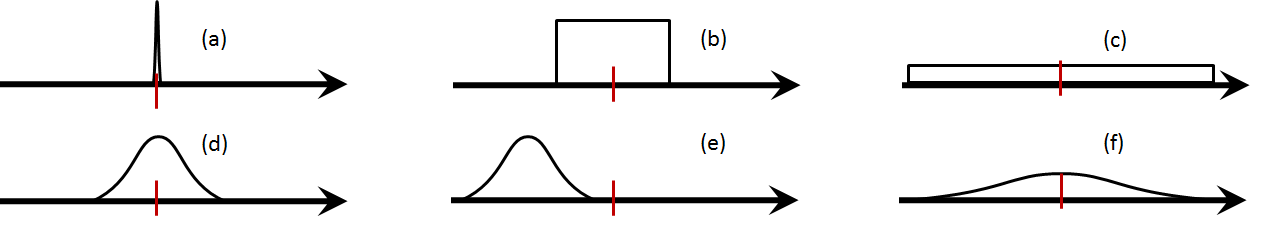
Since the biggest difference between MAP and ML is the addition of the prior \(f_{\mTheta}(\vtheta)\), we need to take a closer look at what they mean. In Figure 8.13 below, we show a set of six different priors. We ask two questions: (1) What do they mean? (2) Which one should we use?
It tells us your belief as to how the underlying parameter \(\mTheta\) should be distributed.
The meaning of this statement can be best understood from the examples shown in Figure 8.13:
- sep0ex
- Figure 8.13(a). This is a delta prior \(f_{\Theta}(\theta) = \delta(\theta)\) (or \(f_{\Theta}(\theta) = \delta(\theta-\theta_0)\)). If you use this prior, you are absolutely sure that the parameter \(\Theta\) takes a specific value. There is no uncertainty about your belief. Since you are so confident about your prior knowledge, you will ignore the likelihood that is constructed from the data. No one will use a delta prior in practice.
- Figure 8.13(b). \(f_{\Theta}(\theta) = \frac{1}{b-a}\) for \(a \le \theta \le b\), and is zero otherwise. This is a bounded uniform prior. You do not have any preference for the parameter \(\Theta\), but you do know from your prior experience that \(a \le \Theta \le b\).
- Figure 8.13(c). This prior is the same as (b) but is short and very wide. If you use this prior, it means that you know nothing about the parameter. So you give up the prior and let the likelihood dominate the MAP estimate.
- Figure 8.13(d). \(f_{\Theta}(\theta) = \text{Gaussian}(0,\sigma^2)\). You use this prior when you know something about the parameter, e.g., that it is centered at certain location and you have some uncertainty.
- Figure 8.13(e). Same as (d), but the parameter is centered at some other location.
- Figure 8.13(f). Same as (d), but you have less confidence about the parameter.
As you can see from these examples, the shape of the prior tells us how you want \(\Theta\) to be distributed. The choice you make will directly influence the MAP optimization, and hence the MAP estimate.
Since the prior is a subjective quantity in the MAP framework, you as the user have the freedom to choose whatever you like. For instance, if you have conducted a similar experiment before, you can use the results of the previous experiments as the current prior. Another strategy is to go with physics. For instance, we can argue that \(\vtheta\) should be sparse so that it contains as few non-zeros as possible. In this case, a sparsity-driven prior, such as \(f_{\mTheta}(\vtheta) = \exp\{-\|\vtheta\|_1\}\), could be a choice. The third strategy is to choose a prior that is computationally “friendlier”, e.g., in quadratic form so that the MAP is differentiable. One such choice is the conjugate prior. We will discuss this later in Section 8.3.6.
- sep0ex
- Based on your preference, e.g., you know from historical data that the parameter should behave in certain ways.
- Based on physics, e.g., the parameter has a physical interpretation, so you need to abide by the physical laws.
- Choose a prior that is computationally “friendlier”. This is the topic of the conjugate prior, which is a prior that does not change the form of the posterior distribution. (We will discuss this later in Section 8.3.6.)
8.3.3MAP formulation and solution
Our next task is to study how to formulate the MAP problem and how to solve it.
Let \(\mX = [X_1,\ldots,X_N]^T\) be i.i.d. observations. Let \(\mTheta\) be a random parameter. The maximum-a-posteriori estimate of \(\mTheta\) is
Philosophically speaking, ML and MAP have two different goals. ML considers a parametric model with a deterministic parameter. Its goal is to find the parameter that maximizes the likelihood for the data we have observed. MAP also considers a parametric model but the parameter \(\mTheta\) is random. Because \(\mTheta\) is random, we are finding one particular state \(\vtheta\) of the parameter \(\mTheta\) that offers the best explanation conditioned on the data \(\mX\) we observe. In a sense, the two optimization problems are
This pair of equations is interesting, as the pair tells us that the difference between the ML estimation and the MAP estimation is the flipped order of \(\mX\) and \(\mTheta\).
There are two reasons we care about the posterior. First, in MAP the posterior allows us to incorporate the prior. ML does not allow a prior. A prior can be useful when the number of samples is small. Second, maximizing the posterior does have some physical interpretations. MAP asks for the probability of \(\mTheta = \vtheta\) after observing \(N\) training samples \(\mX = \vx\). ML asks for the probability of observing \(\mX = \vx\) given a parameter \(\vtheta\). Both are correct and legitimate criteria, but sometimes we might prefer one over the other.
To solve the MAP problem, we notice that
Therefore, what MAP adds is the prior \(\log f_{\mTheta}(\vtheta)\). If you use an uninformative prior, e.g., a prior with extremely wide support, then the MAP estimation will return more or less the same result as the ML estimation.
- sep0ex
- The relation “=” does not make sense here, because \(\vtheta\) is random in MAP but deterministic in ML.
- Solution of MAP optimization = solution of ML optimization, when \(f_{\mTheta}(\vtheta)\) is uniform over the parameter space.
- In this case, \(f_{\mTheta}(\vtheta) = \text{constant}\) and so it can be dropped from the optimization.
Let \(X_1,\ldots,X_N\) be i.i.d. random variables with a PDF \(f_{X_n|\Theta}(x_n|\theta)\) for all \(n\), and \(\Theta\) be a random parameter with PDF \(f_{\Theta}(\theta)\):
Find the MAP estimate.
The MAP estimate is
Since the maximizer is not changed by any monotonic function, we apply logarithm to the above equations. This yields
Constants in the maximization do not matter. So by dropping the constant terms we obtain
It now remains to solve the maximization. To this end we take the derivative w.r.t. \(\theta\) and show that
This yields
Rearranging the terms gives us the final result:
Prove that if \(f_{\mTheta}(\vtheta) = \delta(\vtheta - \vtheta_0)\), the MAP estimate is \(\vthetahat_{\text{MAP}} = \vtheta_0\).
If \(f_{\mTheta}(\vtheta) = \delta(\vtheta - \vtheta_0)\), then
Thus, if \(\vthetahat_{\text{MAP}} \not= \vtheta_0\), the first case says that there is no solution, so we must go with the second case \(\vthetahat_{\text{MAP}} = \vtheta_0\). But if \(\vthetahat_{\text{MAP}} = \vtheta_0\), there is no optimization because we have already chosen \(\vthetahat_{\text{MAP}} = \vtheta_0\). This proves the result.
8.3.4Analyzing the MAP solution
As we said earlier, MAP offers something that ML does not. To see this, we will use the result of the Gaussian random variables as an example and analyze the MAP solution as we change the parameters \(N\) and \(\sigma_0\). Recall that if \(X_1,\ldots,X_N\) are i.i.d. Gaussian random variables with unknown mean \(\theta\) and known variance \(\sigma^2\), the ML estimate is
Assuming that the parameter \(\Theta\) is distributed according to a PDF \(\text{Gaussian}(\mu_0,\sigma_0^2)\), we have shown in the previous subsection that
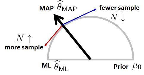
In what follows, we will take a look at the behavior of the MAP estimate \(\thetahat_{\text{MAP}}\) as \(N\) and \(\sigma_0\) change. The results of our discussion are summarized in Figure 8.14.
First, let's look at the effect of \(N\).
}$?}
- sep0ex
- As \(N \rightarrow \infty\), the MAP estimate \(\thetahat_{\text{MAP}} \rightarrow \thetahat_{\text{ML}}\): If we have enough samples, we trust the data.
- As \(N \rightarrow 0\), the MAP estimate \(\thetahat_{\text{MAP}} \rightarrow \mu_0\). If we do not have any samples, we trust the prior.
These two results can be demonstrated by taking the limits. As \(N \rightarrow \infty\), the MAP estimate converges to
This result is not surprising. When we have infinitely many samples, we will completely rely on the data and make our estimate. Thus, the MAP estimate is the same as the ML estimate.
When \(N \rightarrow 0\), the MAP estimate converges to
This means that, when we do not have any samples, the MAP estimate \(\thetahat_{\text{MAP}}\) will completely use the prior distribution, which has a mean \(\mu_0\).
The implication of this result is that MAP offers a natural swing between \(\thetahat_{\text{ML}}\) and \(\mu_0\), controlled by \(N\). Where does this \(N\) come from? If we recall the derivation of the result, we note that the \(N\) affects the likelihood term through the number of samples:
Thus, as \(N\) increases, the influence of the data term grows, and so the result will gradually shift towards \(\thetahat_{\text{ML}}\).
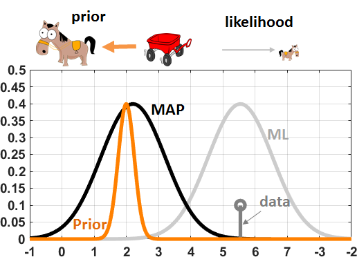
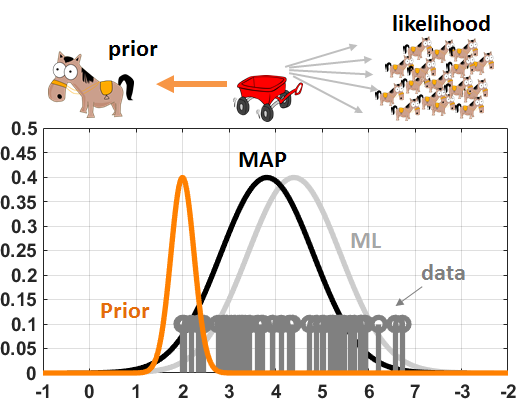
Figure 8.15 illustrates a numerical experiment in which we draw \(N\) random samples \(x_1,\ldots,x_N\) according to a Gaussian distribution \(\text{Gaussian}(\theta,\sigma^2)\), with \(\sigma = 1\). We assume that the prior distribution is \(\text{Gaussian}(\mu_0,\sigma_0^2)\), with \(\mu_0 = 0\) and \(\sigma_0 = 0.25\). The ML estimate of this problem is \(\thetahat_{\text{ML}} = \frac{1}{N}\sum_{n=1}^N x_n\), whereas the MAP estimate is given by Eq. (8.39). The figure shows the resulting PDFs. A helpful analogy is that the prior and the likelihood are pulling a rope in two opposite directions. As \(N\) grows, the force of the likelihood increases and so the influence becomes stronger.
We next look at the effect of \(\sigma_0\).
}$?}
- sep0ex
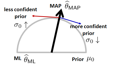
- As \(\sigma_0 \rightarrow \infty\), the MAP estimate \(\thetahat_{\text{MAP}} \rightarrow \thetahat_{\text{ML}}\): If we have doubts about the prior, we trust the data.
- As \(\sigma_0 \rightarrow 0\), the MAP estimate \(\thetahat_{\text{MAP}} \rightarrow \mu_0\). If we are absolutely sure about the prior, we ignore the data.
When \(\sigma_0 \rightarrow \infty\), the limit of \(\thetahat_{\text{MAP}}\) is
The reason why this happens is that \(\sigma_0\) is the uncertainty level of the prior. If \(\sigma_0\) is high, we are not certain about the prior. In this case, MAP chooses to follow the ML estimate.
When \(\sigma_0 \rightarrow 0\), the limit of \(\thetahat_{\text{MAP}}\) is
Note that when \(\sigma_0 \rightarrow 0\), we are essentially saying that we are absolutely sure about the prior. If we are so sure about the prior, there is no need to look at the data. In that case the MAP estimate is \(\mu_0\).
The way to understand the influence of \(\sigma_0\) is to inspect the equation:
Since \(\sigma_0\) is purely a preference you decide, you can control how much trust to put onto the prior.
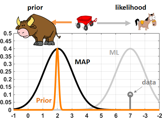
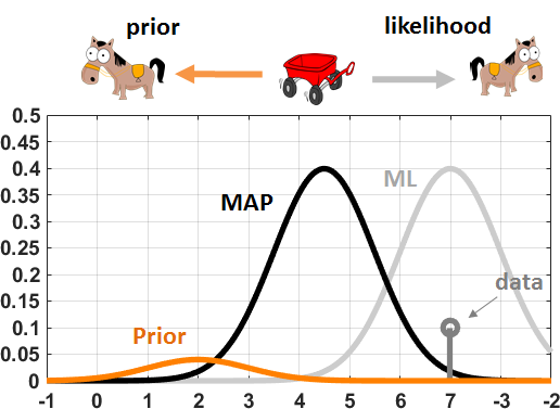
Figure 8.16 illustrates a numerical experiment in which we compare \(\sigma_0 = 0.1\) and \(\sigma_0 = 1\). If \(\sigma_0\) is small, the prior distribution \(f_{\Theta}(\theta)\) becomes similar to a delta function. We can interpret it as a very confident prior, so confident that we wish to align with the prior. The situation can be imagined as a game of tug-of-war between a powerful bull and a horse, which the bull will naturally win. If \(\sigma_0\) is large the prior distribution will become flat. It means that we are not very confident about the prior so that we will trust the data. In this case the MAP estimate will shift towards the ML estimate.
8.3.5Analysis of the posterior distribution
When the likelihood is multiplied with the prior to form the posterior, what does the posterior distribution look like? To answer this question we continue our Gaussian example with a fixed variance \(\sigma\) and an unknown mean \(\theta\). The posterior distribution is proportional to
Performing the multiplication and completing the squares,
where
In other words, the posterior distribution \(f_{\Theta|\mX}(\theta|\vx)\) is also a Gaussian with
If \(f_{\mX|\mTheta}(\vx|\vtheta) = \text{Gaussian}(\vx; \; \theta,\sigma^2)\), and \(f_{\mTheta}(\vtheta) = \text{Gaussian}(\theta ; \; \mu_0,\sigma_0^2)\), what is the posterior \(f_{\mTheta|\mX}(\vtheta|\vx)\)?
The posterior \(f_{\mTheta|\mX}(\vtheta|\vx)\) is \(\text{Gaussian}(\thetahat_{\text{MAP}}, \; \widehat{\sigma}_\text{MAP}^2)\), where
The posterior tells us how \(N\) and \(\sigma_0\) will influence the MAP estimate. As \(N\) grows, the posterior mean and variance become
As a result, the posterior distribution \(f_{\Theta|\mX}(\theta|\vx)\) will converge to a delta function centered at the ML estimate \(\widehat{\theta}_{\text{ML}}\). Therefore, as we try to solve the MAP problem by maximizing the posterior, the MAP estimate has to improve because \(\widehat{\sigma}_\text{MAP} \rightarrow 0\).
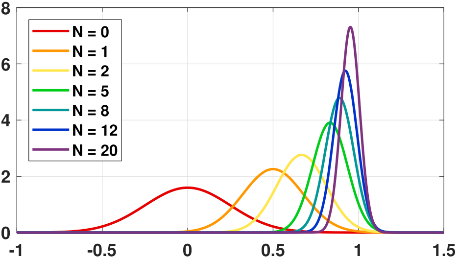
We can plot the posterior distribution \(\text{Gaussian}(\thetahat_{\text{MAP}}, \; \widehat{\sigma}_\text{MAP}^2)\) as a function of the number of samples \(N\). Figure 8.17 illustrates this example using the following configurations. The likelihood is Gaussian with \(\mu = 1\), \(\sigma = 0.25\). The prior is Gaussian with \(\mu_0 = 0\) and \(\sigma_0 = 0.25\). We construct the Gaussian according to \(\text{Gaussian}(\thetahat_{\text{MAP}}, \; \widehat{\sigma}_\text{MAP}^2)\) by varying \(N\). The result shown in Figure 8.17 confirms our prediction: As \(N\) grows, the posterior becomes more like a delta function whose mean is the true mean \(\mu\). The posterior estimator \(\thetahat_{\text{MAP}}\), for each \(N\), is the peak of the respective Gaussian.
- sep0ex
- For every \(N\), MAP has a posterior distribution \(f_{\mTheta|\mX}(\vtheta|\vx)\).
- As \(N\) grows, \(f_{\mTheta|\mX}(\vtheta|\vx)\) converges to a delta function centered at \(\widehat{\vtheta}_{\text{ML}}\).
- MAP tries to find the peak of \(f_{\mTheta|\mX}(\vtheta|\vx)\). For large \(N\), it returns \(\widehat{\vtheta}_{\text{ML}}\).
8.3.6Conjugate prior
Choosing the prior is an important topic in a MAP estimation. We have elaborated two “engineering” solutions: Use your prior experience or follow the physics. In this subsection, we discuss the third option: to choose something computationally friendly. To explain what we mean by “computationally friendly”, let us consider the following example, thanks to Avinash Kak. (Avinash Kak “ML, MAP, and Bayesian — The Holy Trinity of Parameter Estimation and Data Prediction”, https://engineering.purdue.edu/kak/Tutorials/Trinity.pdf)
Consider a Bernoulli distribution with a PDF
To compute the MAP estimate, we assume that we have a prior \(f_{\Theta}(\theta)\). Therefore, the MAP estimate is given by
Let us consider three options for the prior. Which one would you use?
- sep0ex
Candidate 1: \(f_{\Theta}(\theta) = \frac{1}{\sqrt{2\pi \sigma^2}}\exp\left\{-\frac{(\theta-\mu)^2}{2\sigma^2}\right\}\), a Gaussian prior. If you choose this prior, the optimization problem will become
$$\widehat{\theta}_{\text{MAP}} = \argmax{\theta} \;\; \sum_{n=1}^N \bigg\{x_n \log \theta + (1-x_n)\log(1-\theta)\bigg\} - \frac{(\theta-\mu)^2}{2\sigma^2}.$$We can still take the derivative and set it to zero. This gives
$$\begin{aligned} \frac{\sum_{n=1}^N x_n}{\theta} - \frac{N-\sum_{n=1}^N x_n}{1-\theta} = \frac{\theta-\mu}{\sigma^2}. \end{aligned}$$Defining \(S = \sum_{n=1}^N x_n\) and moving the terms around, we have
$$(1-\theta)\sigma^2S - \theta\sigma^2(N-S) = \theta(1-\theta)(\theta-\mu).$$This is a cubic polynomial problem that has a closed-form solution and is also solvable by a computer. But it's also tedious, at least to lazy engineers like ourselves.
Candidate 2: \(f_{\Theta}(\theta) = \frac{\lambda}{2} e^{-\lambda |\theta|}\), a Laplace prior. In this case, the optimization problem becomes
$$\widehat{\theta}_{\text{MAP}} = \argmax{\theta} \;\; \sum_{n=1}^N \bigg\{x_n \log \theta + (1-x_n)\log(1-\theta)\bigg\} - \lambda |\theta|.$$Welcome to convex optimization! There is no closed-form solution. If you want to solve this problem, you need to call a convex solver.
Candidate 3: \(f_{\Theta}(\theta) = \frac{1}{C} \theta^{\alpha-1}(1-\theta)^{\beta-1}\), a beta prior. This prior looks very complicated, but let's plug it into our optimization problem:
$$\begin{aligned} \widehat{\theta}_{\text{MAP}} &=\argmax{\theta} \;\; \sum_{n=1}^N \bigg\{x_n \log \theta \\ &\qquad + (1-x_n)\log(1-\theta)\bigg\} + (\alpha-1)\log\theta + (\beta-1)\log(1-\theta)\\ &= \argmax{\theta} \;\; (S+\alpha-1) \log \theta + (N-S+\beta-1)\log(1-\theta), \end{aligned}$$where \(S = \sum_{n=1}^N x_n\). Taking the derivative and setting it to zero, we have
$$\frac{S+\alpha-1}{\theta} = \frac{N-S+\beta-1}{1-\theta}.$$Rearranging the terms we obtain the final estimate:
$$\widehat{\theta}_{\text{MAP}} = \frac{S+\alpha-1}{N+\beta+\alpha-2}.$$
There are a number of intuitions that we can draw from this beta prior, but most importantly, we have obtained a very simple solution. That is because the posterior distribution remains in the same form as the prior, after multiplying by the prior. Specifically, if we use the beta prior, the posterior distribution is
This is still in the form of \(\theta^{\bigstar-1} (1-\theta)^{\blacksquare-1}\), which is the same as the prior. When this happens, we call the prior a conjugate prior. In this example, the beta prior is a conjugate prior for the Bernoulli likelihood.
- sep0ex
- It is a prior such that when multiplied by the likelihood to form the posterior, the posterior \(f_{\Theta|\mX}(\theta|\vx)\) takes the same form as the prior \(f_{\Theta}(\theta)\).
- Every likelihood has its conjugate prior.
- Conjugate priors are not necessarily good priors. They are just computationally friendly. Some of them have good physical interpretations.
We can make a few interpretations of the beta prior, in the context of Bernoulli likelihood. First, the beta distribution takes the form
where \(B(\alpha,\beta)\) is the beta function (The beta function is defined as \(B(\alpha,\beta) = \frac{\Gamma(\alpha)\Gamma(\beta)}{\Gamma(\alpha+\beta)}\), where \(\Gamma\) is the gamma function. For integer \(n\), \(\Gamma(n) = (n-1)!\)). The shape of the beta distribution is shown in Figure 8.18. For different choices of \(\alpha\) and \(\beta\), the distribution has a peak located towards either side of the interval \([0,1]\). For example, if \(\alpha\) is large but \(\beta\) is small, the distribution \(f_{\Theta}(\theta)\) leans towards 1 (the yellow curve).
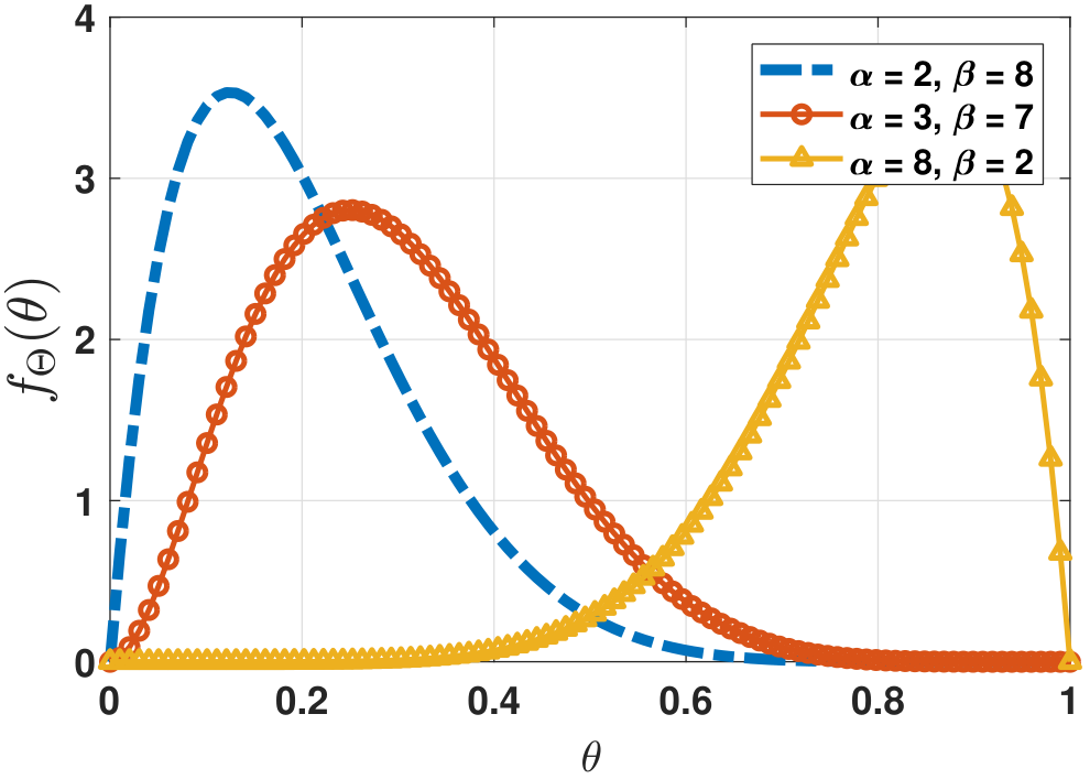
As a user, you have the freedom to pick \(f_{\Theta}(\theta)\). Even if you are restricted to the beta distribution, you still have plenty of degrees of freedom in choosing \(\alpha\) and \(\beta\) so that your choice matches your belief. For example, if you know ahead of time that the Bernoulli experiment is biased towards 1 (e.g., the coin is more likely to come up heads), you can choose a large \(\alpha\) and a small \(\beta\). By contrast, if you believe that the coin is fair, you choose \(\alpha = \beta\). The parameters \(\alpha\) and \(\beta\) are known as the hyperparameters of the prior distribution. Hyperparameters are parameters for \(f_{\Theta}(\theta)\).
(Prior for Gaussian mean) Consider a Gaussian likelihood for a fixed variance \(\sigma^2\) and unknown mean \(\theta\):
Show that the conjugate prior is given by
We have shown this result previously. By some (tedious) completing squares, we show that
where
Since \(f_{\Theta|\mX}(\theta|\vx)\) is in the same form as \(f_{\Theta}(\theta)\), we know that \(f_{\Theta}(\theta)\) is a conjugate prior.
(Prior for Gaussian variance) Consider a Gaussian likelihood for a mean \(\mu\) and unknown variance \(\sigma^2\):
Find the conjugate prior.
We first define the precision \(\theta = \frac{1}{\sigma^2}\). The likelihood is
We propose to choose the prior \(f_{\Theta}(\theta)\) as
for some \(a\) and \(b\). This \(f_{\Theta}(\theta)\) is called the Gamma distribution \(\text{Gamma}(\theta|a,b)\). We can show that \(\E[\Theta] = \frac{a}{b}\) and \(\Var[\Theta] = \frac{a}{b^2}\). With some (tedious) completing squares, we show that the posterior is
which is in the same form as the prior. So we know that our proposed \(f_{\Theta}(\theta)\) is a conjugate prior.
The story of conjugate priors is endless because every likelihood has its conjugate prior. Table 8.1 summarizes a few commonly used conjugate priors, their likelihoods, and their posteriors. The list can be expanded further to distributions with multiple parameters. For example, if a Gaussian has both unknown mean and variance, then there exists a conjugate prior consisting of a Gaussian multiplied by a Gamma. Conjugate priors also apply to multidimensional distributions. For example, the prior for the mean vector of a high-dimensional Gaussian is another high-dimensional Gaussian. The prior for the covariance matrix of a high-dimensional Gaussian is the Wishart prior. The prior for both the mean vector and the covariance matrix is the normal Wishart.
| Table of Conjugate Priors | ||
| Likelihood | Conjugate Prior | Posterior |
| \(f_{\mX|\Theta}(\vx|\theta)\) | \(f_{\Theta}(\theta)\) | \(f_{\Theta|\mX}(\theta|\vx)\) |
| \(\text{Bernoulli}(\theta)\) | \(\text{Beta}(\alpha,\beta)\) | \(\text{Beta}(\alpha + S, \beta+N-S)\) |
| \(\text{Poisson}(\theta)\) | \(\text{Gamma}(\alpha,\beta)\) | \(\text{Gamma}\left(\alpha+S,\ \beta+N\right)\) |
| \(\text{Exponential}(\theta)\) | \(\text{Gamma}(\alpha,\beta)\) | \(\text{Gamma}\left(\alpha+N,\ \beta+S\right)\) |
| \(\text{Gaussian}(\theta,\sigma^2)\) | \(\text{Gaussian}(\mu_0,\sigma_0^2)\) | \(\text{Gaussian}\left(\frac{\mu_0/\sigma_0^2+S/\sigma^2}{1/\sigma_0^2+N/\sigma^2}, \frac{1}{\frac{N}{\sigma^2}+\frac{1}{\sigma_0^2}}\right)\) |
| \(\text{Gaussian}(\mu,\theta^2)\) | \(\text{Inv. Gamma}(\alpha,\beta)\) | \(\text{Inv. Gamma}\left(\alpha+\tfrac{N}{2}, \beta+\tfrac{1}{2}\sum_{n=1}^N (x_n-\mu)^2\right)\) |
8.3.7Linking MAP with regression
ML and regression represent the statistics and the optimization aspects of the same problem. With the parallel argument, MAP is linked to the regularized regression. The reason follows immediately from the definition of MAP:
To make this more explicit, we consider the following linear regression problem:
If we assume that \(\ve \sim \text{Gaussian}(0,\sigma^2\mI)\), the likelihood is defined as
In the ML setting, the ML estimate is the maximizer of the likelihood:
For MAP, we add a prior term so that the optimization becomes
Therefore, the regularization of the regression is exactly \(-\log f_{\mTheta}(\vtheta)\). We can perform reverse engineering to find out the corresponding prior for our favorite choices of the regularization.
Ridge regression. Suppose that
Taking the negative log on both sides yields
Putting this into the MAP estimate,
where \(\lambda\) is the corresponding ridge regularization parameter. Therefore, the ridge regression is equivalent to a MAP estimation using a Gaussian prior.
- sep0ex
In MAP, define the prior as a Gaussian:
$$f_{\mTheta}(\vtheta) = \exp\left\{-\frac{\|\vtheta\|^2}{2\sigma_0^2}\right\}.$$- The prior says that the solution \(\vtheta\) is naturally distributed according to a Gaussian with mean zero and variance \(\sigma_0^2\).
LASSO regression. Suppose that
Taking the negative log on both sides yields
Putting this into the MAP estimate we can show that
To summarize:
- sep0ex
LASSO is a MAP using the prior
$$f_{\mTheta}(\vtheta) = \exp\left\{-\frac{\|\vtheta\|_1}{\alpha}\right\}.$$
At this point, you may be wondering what MAP buys us when regularized regression can already do the job. The answer is about the interpretation. While regularized regression can always return us a result, that is just a result. However, if you know that the parameter \(\vtheta\) is distributed according to some distributions \(f_{\mTheta}(\vtheta)\), MAP offers a statistical perspective of the solution in the sense that it returns the peak of the posterior \(f_{\mTheta|\mX}(\vtheta|\vx)\). For example, if we know that the data is generated from a linear model with Gaussian noise, and if we know that the true regression coefficients are drawn from a Gaussian, then the ridge regression is guaranteed to be optimal in the posterior sense. Similarly, if we know that there are outliers and have some ideas about the outlier statistics, perhaps the LASSO regression is a better choice.
It is also important to note the different optimalities offered by MAP versus ML versus regression. The optimality offered by regression is the training loss, which can always give us a result even if the underlying statistics do not match the optimization formulation, e.g., there are outliers, and you use unregularized least-squares minimization. You can get a result, but the outliers will heavily influence your solution. On the other hand, if you know the data statistics and choose to follow the ML, then the ML solution is optimal in the sense of optimizing the likelihood \(f_{\mX|\mTheta}(\vx|\vtheta)\). If you further know the prior statistics, the MAP solution will be optimal, but this time it is optimal w.r.t. the posterior \(f_{\mTheta|\mX}(\vtheta|\vx)\). Since each of these is optimizing for a different goal, they are only good for their chosen objectives. For example, \(\widehat{\vtheta}_{\text{MAP}}\) can be a biased estimate if our goal is to maximize the likelihood. The \(\widehat{\vtheta}_{\text{ML}}\) is optimal for the likelihood but can be a bad choice for the posterior. Both \(\widehat{\vtheta}_{\text{MAP}}\) and \(\widehat{\vtheta}_{\text{ML}}\) can possibly achieve a reasonable mean-squared error, but their results may not make sense (e.g., if \(\vtheta\) is an image then \(\widehat{\vtheta}_{\text{MAP}}\) may over-smooth the image whereas \(\widehat{\vtheta}_{\text{ML}}\) amplifies noise). So it's incorrect to think that \(\widehat{\vtheta}_{\text{MAP}}\) is superior to \(\widehat{\vtheta}_{\text{ML}}\) because it is more general.
Here are some rules of thumb for MAP, ML, and regression:
- sep0ex
- Regression: If you are lazy and you know nothing about the statistics, do the regression with whatever regularization you prefer. It will give you a result. See if it makes sense with your data.
- MAP: If you know the statistics of the data, and if you have some preference for the prior distribution, go with MAP. It will offer you the optimal solution w.r.t. finding the peak of the posterior.
- ML: If you are interested in some simple-form solution, and you want those nice properties such as consistency and unbiasedness, then go with ML. It usually possesses the “friendly” properties so that you can derive the performance limit.