eBook › Chapter 8 · Estimation

Section 8.4

Minimum Mean-Square Estimation

First-time readers are often tempted to think that the maximum-likelihood estimation or the maximum a posteriori estimation is the best method to estimate parameters. In some sense, this is true because both estimation procedures offer some form of optimal explanation for the observed variables. However, as we said above, being optimal with respect to the likelihood or the posterior only means optimal under the respective criteria. An ML estimate is not necessarily optimal for the posterior, whereas a MAP estimate is not necessarily optimal for the likelihood. Therefore, as we proceed to the third commonly used estimation strategy, we need to remind ourselves of the specific type of optimality we seek.

8.4.1Positioning the minimum mean-square estimation

Mean-square error estimation, as it is termed, uses the mean-square error as the optimality criterion. The corresponding estimation process is known as the minimum mean-square estimation (MMSE). MMSE is a Bayesian approach, meaning that it uses the prior $f_{\mTheta}(\vtheta)$ as well as the likelihood $f_{\mX|\mTheta}(\vx|\vtheta)$. As we will show shortly, the MMSE estimate of a set of i.i.d. observations $\mX = [X_1,\ldots,X_N]^T$ is

\begin{aligned} \vthetahat_{\text{MMSE}}(\vx) &\overset{(a)}{=} \E_{\mTheta|\mX}\left[ \mTheta | \mX = \vx\right] \qquad\qquad (a): \text{We will discuss this.}\\ &= \int \vtheta \cdot f_{\mTheta|\mX}(\vtheta|\vx)\, d\vtheta. \end{aligned}

You may find this equation very surprising, because it says that the MMSE estimate is the mean of the posterior distribution $f_{\mTheta|\mX}(\vtheta|\vx)$. Let's compare this result with the ML estimate and the MAP estimate:

\begin{aligned} &\vthetahat_{\text{ML}} = \text{peak of } f_{\mX|\mTheta}(\vx \;|\; \vtheta),\\ &\vthetahat_{\text{MAP}} = \text{peak of } f_{\mTheta|\mX}(\vtheta \;|\; \vx),\\ &\vthetahat_{\text{MMSE}} = \text{average of } f_{\mTheta|\mX}(\vtheta \;|\; \vx). \end{aligned}

Therefore, an MMSE estimate is not by any means universally superior or inferior to a MAP estimate or an ML estimate. It is just a different estimate with a different goal.

So how exactly are these estimates different? Figure 8.19 illustrates a typical situation of asymmetric distribution. Here, we plot both the likelihood function $f_{\mX|\mTheta}(\vx \;|\; \vtheta)$ and the posterior function $f_{\mTheta|\mX}(\vtheta \;|\; \vx)$.

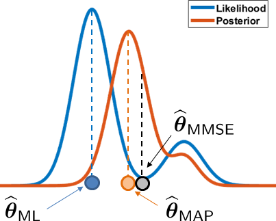
As shown in the figure, the ML estimate is the peak of the likelihood, whereas the MAP estimate is the peak of the posterior. The third estimate is the MMSE estimate, which is the average of the posterior distribution. It is easy to see that if the posterior distribution is symmetric and has a single peak, the peak is always the mean. Therefore, for single-peak symmetric distributions, MMSE and MAP estimates are identical.

What is so special about the MMSE estimate?

sep0ex
MMSE is a Bayesian estimation, so it requires a prior.
An MMSE estimate is the mean of the posterior distribution.
MMSE estimate = MAP estimate if the posterior distribution is symmetric and has a single peak.

8.4.2Mean squared error

The MMSE is based on minimizing the mean squared error (MSE). In this subsection we discuss the mean squared error in the Bayesian setting. In the deterministic setting, given an estimate $\thetahat$ and a ground truth $\theta$, the MSE is defined as

\text{MSE}( \underset{\text{\textcolor{blue}{ground truth}}}{\underbrace{\quad \theta \quad}} , \underset{\text{\textcolor{blue}{estimate}}}{\underbrace{\quad \thetahat \quad}} ) = (\theta- \thetahat)^2.

In any estimation problem, the estimate $\thetahat$ is always a function of the observed variables. Thus, we have

\thetahat(\mX) = g(\mX), \qquad\mbox{where}\qquad \mX = [X_1,\ldots,X_N]^T,

for some function $g(\cdot)$. Substituting this into the definition of MSE, and recognizing that $\mX$ is drawn from a distribution $f_{\mX}(\vx)$, we take the expectation to define the MSE as

\begin{aligned} \text{MSE}(\theta,\thetahat) &= (\theta-\thetahat)^2\\ &\Downarrow \textcolor{blue}{\text{\footnotesize{replace $\thetahat$ by $g(\mX)$}}}\\ \text{MSE}(\theta,\thetahat) &= (\theta-\textcolor{blue}{g(\mX)})^2\\ &\Downarrow \textcolor{blue}{\text{\footnotesize{take expectation over $\mX$}}}\\ \text{MSE}(\theta,\thetahat) &= \textcolor{blue}{\E_{\mX}}\left[(\theta-g(\mX))^2\right]. \end{aligned}

Thus we have arrived at the definition of MSE. We call this the frequentist version, because the parameter $\theta$ is deterministic.

Definition 8.8 (Mean squared error, frequentist)

The mean squared error of an estimate $g(\mX)$ w.r.t. the true parameter $\theta$ is

\text{MSE}_{\text{freq}}(\theta,g(\cdot)) = \E_{\mX}\left[(\theta - g(\mX))^2\right].

If the parameter $\vtheta$ is high-dimensional, so is the estimate $\vg(\mX)$, and the MSE is

\text{MSE}_{\text{freq}}(\vtheta,\vg(\cdot)) = \E_{\mX}\left[\|\vtheta - \vg(\mX)\|^2\right].

Note that in the above definition the MSE is measured between the true parameter $\theta$ and the estimator $g(\cdot)$. We use the function $g(\cdot)$ here because we have taken the expectation of all the possible inputs $\mX$. So we are not comparing $\theta$ with a value $g(\mX)$ but with the function $g(\cdot)$.

If we take a Bayesian approach such as the MAP, then $\theta$ itself is a random variable $\Theta$. To compute the MSE, we then need to take the average across all the possible choices of ground truth $\Theta$. This leads to

\begin{aligned} \text{MSE}(\theta,\thetahat) &= \textcolor{blue}{\E_{\mX}}\left[(\theta-g(\mX))^2\right]\\ &\Downarrow \textcolor{blue}{\text{\footnotesize{replace $\theta$ by $\Theta$}}}\\ \text{MSE}(\theta,\thetahat) &= \E_{\mX}\left[(\textcolor{blue}{\Theta}-g(\mX))^2\right]\\ &\Downarrow \textcolor{blue}{\text{\footnotesize{take expectation over $\Theta$}}}\\ \text{MSE}(\theta,\thetahat) &= \textcolor{blue}{\E_{\mX,\Theta}}\left[(\Theta-g(\mX))^2\right]. \end{aligned}

Therefore, we have arrived at our definition of the MSE, in the Bayesian setting.

Definition 8.9 (Mean squared error, Bayesian)

The mean squared error of an estimate $g(\mX)$ w.r.t. the true parameter $\Theta$ is

\text{MSE}_{\text{Bayes}}(\Theta,g(\cdot)) = \E_{\Theta,\mX}\left[(\Theta - g(\mX))^2\right].

If the parameter $\mTheta$ is high-dimensional, so is the estimate $\vg(\mX)$, and the MSE is

\text{MSE}_{\text{Bayes}}(\mTheta,\vg(\cdot)) = \E_{\mTheta,\mX}\left[\|\mTheta - \vg(\mX)\|^2\right].

The difference between the Bayesian MSE and the frequentist MSE is the expectation over $\Theta$. Practically speaking, the frequentist MSE is more of an evaluation metric than an objective function for solving an inverse problem. The reason is that in an inverse problem, we never have access to the true parameter $\theta$. (If we knew $\theta$, there would be no problem to solve.) Bayesian MSE is more meaningful. It says that we do not know the true parameter $\theta$, but we know its statistics. We are trying to find the best $g(\cdot)$ that minimizes the error. Our solution will depend on the statistics of $\Theta$ but not on the unknown true parameter $\theta$.

When we say minimum mean squared error, we typically refer to the Bayesian MMSE. In this case, the problem we solve is

g(\cdot) = \argmin{g(\cdot)} \; \E_{\Theta,\mX}\left[(\Theta - g(\mX))^2\right].

As you can see from Definition 8.9, the goal of the Bayesian MMSE is to find a function $g: \R^N \rightarrow \R$ such that the joint expectation $\E_{\Theta,\mX}\left[(\Theta - g(\mX))^2\right]$ is minimized. In the case where $\mTheta$ is a vector, the problem becomes

\vg(\cdot) = \argmin{\vg(\cdot)} \;\; \E_{\mTheta,\mX}\left[\|\mTheta - \vg(\mX)\|^2\right],

where $\vg(\cdot): \R^{N\times d} \rightarrow \R^d$ if $\mTheta$ is a $d$-dimensional vector. The function $\vg$ will take a sequence of $N$ observed numbers and estimate the parameter $\mTheta$.

What is the Bayesian MMSE estimate?

The Bayesian MMSE estimate is obtained by minimizing the MSE:

g(\cdot) = \argmin{g(\cdot)} \;\; \E_{\Theta,\mX}\left[(\Theta - g(\mX))^2\right].

8.4.3MMSE estimate = conditional expectation

Theorem 8.2

The Bayesian MMSE estimate is

\begin{aligned} \thetahat_{\text{MMSE}} &= \argmin{g(\cdot)} \;\; \E_{\Theta,\mX}\left[(\Theta - g(\mX))^2\right] \\ &= \E_{\Theta|\mX}[\Theta \;|\; \mX = \vx]. \end{aligned}

Proof. First of all, we decompose the joint expectation:

\begin{aligned} \E_{\Theta,\mX}\left[(\Theta - g(\mX))^2\right] &= \int \E_{\Theta|\mX}\left[(\Theta - g(\mX))^2 \; | \; \mX = \vx \right] f_{\mX}(\vx)\, d\vx. \end{aligned}

Since $f_{\mX}(\vx) \ge 0$ for all $\vx$, and $\E_{\Theta|\mX}\left[(\Theta - g(\mX))^2 \; | \; \mX = \vx \right] \ge 0$ because it is a square, it follows that the integral is minimized when $\E_{\Theta|\mX}\left[(\Theta - g(\mX))^2 \; | \; \mX = \vx \right]$ is minimized.

The conditional expectation can be evaluated as

\begin{aligned} &\E_{\Theta|\mX}[(\Theta - g(\mX))^2 \; | \; \mX = \vx]\\ &= \E_{\Theta|\mX} \bigg[\Theta^2 - 2\Theta g(\mX) + g(\mX)^2 \; \bigg| \; \mX = \vx \bigg]\\ &= \underset{\bydef V(\vx)}{\underbrace{\E_{\Theta|\mX} \bigg[\Theta^2 \; \Big| \; \mX = \vx \bigg]}} - 2\underset{\bydef u(\vx)}{\underbrace{\E_{\Theta|\mX} \bigg[ \Theta \; \Big| \; \mX = \vx \bigg]}}g(\vx) + g(\vx)^2 \\ &= V(\vx) - 2u(\vx) g(\vx) + g(\vx)^2 + \textcolor{blue}{u(\vx)^2-u(\vx)^2}\\ &= V(\vx) - u(\vx)^2 + (u(\vx) - g(\vx))^2\\ &\ge V(\vx) - u(\vx)^2, \qquad \forall g(\cdot), \end{aligned}

where the last inequality holds because no matter what $g(\cdot)$ we choose, the square term $(u(\vx) - g(\vx))^2$ is non-negative. Therefore, $\E_{\Theta|\mX}[(\Theta - g(\mX))^2 \; | \; \mX = \vx]$ is lower-bounded by $V(\vx) - u(\vx)^2$, which is a bound that is independent of $g(\cdot)$. If we can find a $g(\cdot)$ such that this lower bound can be met, the corresponding $g(\cdot)$ is the minimizer.

To this end we only need to make $\E_{\Theta|\mX}[(\Theta - g(\mX))^2 \; | \; \mX = \vx]$ equal $V(\vx) - u(\vx)^2$, but this is easy: the equality holds if and only if $(u(\vx) - g(\vx))^2 = 0$. In other words, if we choose $g(\cdot)$ such that $g(\vx) = u(\vx)$, the corresponding $g(\cdot)$ is the minimizer. This $g(\cdot)$, by substituting the definition of $u(\vx)$, is

g(\vx) = \E_{\Theta|\mX} \bigg[ \Theta \; \Big| \; \mX = \vx \bigg].

This completes the proof.

■

What is the MMSE estimate?

The MMSE estimate is

\thetahat_{\text{MMSE}}(\vx) = \E_{\Theta|\mX}[\Theta \;|\; \mX = \vx].

We emphasize that $\thetahat_{\text{MMSE}}(\vx)$ is a function of $\vx$, because for a different set of observations $\vx$ we will have a different estimated value. Since $\vx$ is a random realization of the random vector $\mX$, we can also define the MMSE estimator as

\Thetahat_{\text{MMSE}}(\mX) = \E_{\Theta|\mX}[\Theta \;|\; \mX].

In this notation, we emphasize that the estimator $\Thetahat_{\text{MMSE}}$ returns a random parameter. The input to the estimator is the random vector $\mX$. Because we are not looking at a particular realization $\mX = \vx$ but the general $\mX$, $\Thetahat_{\text{MMSE}}$ is a function of $\mX$ and not $\vx$.

Conditional expectation of what?

An MMSE estimator is the conditional expectation of $\Theta$ given $\mX = \vx$:

\E_{\Theta|\mX} \bigg[ \Theta \; \Big| \; \mX = \vx \bigg] = \int \theta \; f_{\Theta|\mX}(\theta|\vx)\, d\theta.

This is the expectation using the posterior distribution $f_{\Theta|\mX}(\theta|\vx)$. It should be compared to the peak of the posterior, which returns us the MAP estimate. The posterior distribution is constructed through Bayes' theorem:

f_{\Theta|\mX}(\theta|\vx) = \frac{f_{\mX|\Theta}(\vx|\theta) f_{\Theta}(\theta) }{f_{\mX}(\vx)}.

Therefore, to evaluate the expectation of the condition distribution, we need to include the normalization constant $f_{\mX}(\vx)$, which was omitted in MAP.

The discussion about the mean squared error and the vector estimates can be skipped if this is your first time reading the book.

What is the mean squared error when using the MMSE estimator?

sep0ex
The mean squared error conditioned on the observation is
$\begin{aligned} \text{MSE}(\Theta,\Thetahat_{\text{MMSE}}(\mX)) &\bydef \E_{\Theta|\mX}[(\Theta - \Thetahat_{\text{MMSE}}(\mX))^2 \; | \; \mX] \\ &= \text{Var}_{\Theta|\mX}[\Theta | \mX], \end{aligned}$
which is the conditional variance.
The overall mean squared error, unconditioned, is
$\begin{aligned} \text{MSE}(\Theta,\Thetahat_{\text{MMSE}}(\cdot)) &= \E_{\mX}\left[\text{Var}_{\Theta|\mX}[\Theta | \mX]\right]. \end{aligned}$

Proof. Let us prove these two statements. The resulting MSE is obtained by substituting $\Thetahat_{\text{MMSE}}(\vx) = \E_{\Theta|\mX} \big[ \Theta \; \big| \; \mX \big]$ into the $\text{MSE}(\Theta,\Thetahat_{\text{MMSE}}(\mX))$. To this end, we have that

\begin{aligned} \E_{\Theta|\mX}[(\Theta - \Thetahat_{\text{MMSE}}(\mX))^2 \; | \; \mX] &= V(\mX) - u(\mX)^2 \\ &\qquad \qquad + \underset{\textcolor{blue}{=0, \; \text{because} \; \Thetahat_{\text{MMSE}}(\mX) = \E_{\Theta|\mX}[\Theta|\mX] = u(\mX)}}{\underbrace{\qquad (u(\mX) - \Thetahat_{\text{MMSE}}(\mX))^2 \qquad }}. \end{aligned}

The variables $V$ and $u$ are defined as

\begin{aligned} V(\mX) &= \E_{\Theta|\mX} \big[\Theta^2 \; \Big| \; \mX \big] = \text{2nd moment of $\Theta$ using } f_{\Theta|\mX}(\theta|\vx),\\ u(\mX) &= \E_{\Theta|\mX} \big[ \Theta \; \big| \; \mX \big] = \text{1st moment of $\Theta$ using } f_{\Theta|\mX}(\theta|\vx). \end{aligned}

Since $\Var[Z] = \E[Z^2]-\E[Z]^2$ for any random variable $Z$, it follows that

\begin{aligned} \E_{\Theta|\mX}[(\Theta - \Thetahat_{\text{MMSE}}(\mX))^2 \; | \; \mX] &= V(\mX) - u(\mX)^2 \\ &= \E_{\Theta|\mX} \big[\Theta^2 \; \Big| \; \mX \big] - \left(\E_{\Theta|\mX} \big[ \Theta \; \big| \; \mX \big]\right)^2\\ &= \text{variance of $\Theta$ using } f_{\Theta|\mX}(\theta|\vx)\\ &\bydef \text{Var}_{\Theta|\mX}[\Theta | \mX]. \end{aligned}

Substituting this conditional variance into the MSE definition,

\begin{aligned} \text{MSE}(\Theta,\Thetahat_{\text{MMSE}}(\cdot)) &= \int \E_{\Theta|\mX}[(\Theta - \Thetahat_{\text{MMSE}}(\mX))^2 \; | \; \mX = \vx] f_{\mX}(\vx)\, d\vx \\ &= \int \text{Var}_{\Theta|\mX}[\Theta | \mX = \vx] f_{\mX}(\vx)\, d\vx. \end{aligned}

■

What happens if the parameter is a vector?

sep0ex
The MMSE estimate is $\vthetahat_{\text{MMSE}}(\vx) = \E_{\mTheta|\mX}[\mTheta|\mX = \vx]$.
The MSE is
$\begin{aligned} \text{MSE}(\mTheta,\mThetahat_{\text{MMSE}}(\cdot)) &= \text{Tr} \bigg\{\E_{\mX} \Big\{\text{Cov}(\mTheta|\mX)\Big\}\bigg\}. \end{aligned}$

Proof. The first statement, that the MMSE estimate is

\vthetahat_{\text{MMSE}}(\vx) = \E_{\mTheta|\mX}[\mTheta|\mX = \vx],

is easy to understand since it just follows from the scalar case. The estimator is $\mThetahat_{\text{MMSE}}(\mX) = \E_{\mTheta|\mX}[\mTheta|\mX]$. The corresponding MSE is

\begin{aligned} \text{MSE}(\mTheta,\mThetahat_{\text{MMSE}}(\cdot)) &= \E_{\mTheta, \mX}[\|\mTheta - \mThetahat_{\text{MMSE}}(\mX)\|^2]\\ &= \E_{\mX} \bigg\{\E_{\mTheta| \mX}[\|\mTheta - \mThetahat_{\text{MMSE}}(\mX)\|^2 \;|\; \mX ]\bigg\}, \end{aligned}

where we have used the law of total expectation to decompose the joint expectation. Using the matrix identity below, we have that

\begin{aligned} &\E_{\mX} \bigg\{\E_{\mTheta| \mX}[\|\mTheta - \mThetahat_{\text{MMSE}}(\mX)\|^2 \;|\; \mX ]\bigg\}\\ &= \E_{\mX} \bigg\{\E_{\mTheta|\mX}\Big[ \text{Tr} \left\{(\mTheta - \mThetahat_{\text{MMSE}}(\mX))(\mTheta - \mThetahat_{\text{MMSE}}(\mX))^T\right\} \; | \; \mX \Big]\bigg\}\\ &= \text{Tr} \left\{\E_{\mX} \bigg\{\E_{\mTheta|\mX}\Big[ (\mTheta - \mThetahat_{\text{MMSE}}(\mX))(\mTheta - \mThetahat_{\text{MMSE}}(\mX))^T \; | \; \mX \Big]\bigg\}\right\}. \end{aligned}

However, since the MMSE estimator is the conditional expectation of the posterior, it follows that the inner expectation is the conditional covariance. Therefore, we arrive at the second statement:

\begin{aligned} \text{MSE}(\mTheta,\mThetahat_{\text{MMSE}}(\cdot)) &= \text{Tr} \left\{\E_{\mX} \bigg\{\E_{\mTheta|\mX}\Big[ (\mTheta - \mThetahat_{\text{MMSE}}(\mX))(\mTheta - \mThetahat_{\text{MMSE}}(\mX))^T \; | \; \mX \Big]\bigg\}\right\}\\ &= \text{Tr} \bigg\{\E_{\mX} \Big\{\text{Cov}(\mTheta|\mX)\Big\}\bigg\}. \end{aligned}

■

To prove the two statements above, we need some tools from linear algebra. The two specific matrix identities are given by the following lemma:

Lemma 8.1

The following are matrix identities:

sep0ex
For any random vector $\mTheta \in \R^d$,
$\|\mTheta\|^2 = \text{Tr}(\mTheta^T\mTheta) = \text{Tr}(\mTheta\mTheta^T).$
For any random vector $\mTheta \in \R^d$,
$\E_{\mTheta}[\text{Tr}(\mTheta\mTheta^T)] = \text{Tr}(\E_{\mTheta}[\mTheta\mTheta^T]).$

The proof of these two results is straightforward. The first is due to the cyclic property of the trace operator. The second statement is true because the trace is a linear operator that sums the diagonal of a matrix.

The end of the discussion. Please join us again.

Example 8.22

Let

\begin{aligned} f_{X|\Theta}(x|\theta) = \begin{cases} \theta e^{-\theta x}, &\qquad x \ge 0,\\ 0, &\qquad x < 0, \end{cases} \qquad\text{and}\qquad f_{\Theta}(\theta) = \begin{cases} \alpha e^{-\alpha \theta}, &\qquad \theta \ge 0,\\ 0, &\qquad \theta < 0. \end{cases} \end{aligned}

Find the ML, MAP, and MMSE estimates for a single observation $X = x$.

Solution

We first find the posterior distribution:

\begin{aligned} f_{\Theta|X}(\theta|x) &= \frac{f_{X|\Theta}(x|\theta) f_{\Theta}(\theta) }{ f_X(x)}\\ &= \frac{\alpha \theta e^{-(\alpha+x)\theta}}{\int_0^\infty \alpha \theta e^{-(\alpha+x)\theta} \; d\theta} \\ &= \frac{\alpha \theta e^{-(\alpha+x)\theta}}{\frac{\alpha}{(\alpha+x)^2}}\\ &= (\alpha+x)^2 \theta e^{-(\alpha+x)\theta}. \end{aligned}

The MMSE estimate is the conditional expectation of the posterior:

\begin{aligned} \thetahat_{\text{MMSE}}(x) &= \E_{\Theta|X}[\Theta|X = x] \\ &= \int_0^\infty \theta f_{\Theta|X}(\theta|x) \; d\theta\\ &= \int_0^\infty \theta (\alpha+x)^2 \theta e^{-(\alpha+x)\theta} \; d\theta\\ &= (\alpha+x) \underset{\textcolor{blue}{\text{2nd moment of exponential distribution}}}{\underbrace{ \int_0^\infty \theta^2 \cdot (\alpha+x) e^{-(\alpha+x)\theta} \; d\theta}} \\ &= (\alpha+x) \cdot \frac{2}{(\alpha+x)^2} = \frac{2}{\alpha+x}. \end{aligned}

The MAP estimate is the peak of the posterior:

\begin{aligned} \thetahat_{\text{MAP}}(x) &= \argmax{\theta} \quad \log f_{X|\Theta}(x|\theta) + \log f_{\Theta}(\theta)\\ &= \argmax{\theta} \quad -\theta x + \log \theta - \alpha \theta + \log \alpha. \end{aligned}

Taking the derivative and setting it to zero yields $-x + \frac{1}{\theta} - \alpha = 0$. This implies that

\begin{aligned} \thetahat_{\text{MAP}}(x) = \frac{1}{\alpha+x}. \end{aligned}

Finally, the ML estimate is

\begin{aligned} \thetahat_{\text{ML}}(x) &= \argmax{\theta} \quad \log f_{X|\Theta}(x|\theta) = \frac{1}{x}. \end{aligned}

Practice Exercise 8.8

Following the previous example, derive the estimates for multiple observations $\mX = \vx$.

Solution

The posterior is

\begin{aligned} f_{\Theta|\mX}(\theta|\vx) &= \frac{f_{\mX|\Theta}(\vx|\theta) f_{\Theta}(\theta) }{ f_{\mX}(\vx)}\\ &= \frac{ (\prod_{n=1}^N f_{X|\Theta}(x_n|\theta) )f_{\Theta}(\theta) }{ f_{\mX}(\vx)} \\ &= \frac{ \alpha \theta^N e^{-(\alpha+\sum_{n=1}^N x_n)\theta} }{ \int_0^\infty \alpha \theta^N e^{-(\alpha+\sum_{n=1}^N x_n)\theta} \; d\theta } \\ &= \frac{\left(\alpha+\sum_{n=1}^N x_n \right)^{N+1}}{N!} \theta^N e^{-\left(\alpha+\sum_{n=1}^N x_n\right)\theta}. \end{aligned}

Therefore, the posterior is $\text{Gamma}(N+1,\, \alpha+\sum_{n=1}^N x_n)$. Hence, the estimates are:

\begin{aligned} \thetahat_{\text{MMSE}}(x) &= \frac{N+1}{\alpha+\sum_{n=1}^N x_n},\\ \thetahat_{\text{MAP}}(x) &= \frac{N}{\alpha+\sum_{n=1}^N x_n},\\ \thetahat_{\text{ML}}(x) &= \frac{N}{\sum_{n=1}^N x_n}. \end{aligned}

For finite $N$, the MAP estimate is offset from the ML estimate by the prior parameter $\alpha$ in its denominator. However, as $N \rightarrow \infty$ the posterior is dominated by the likelihood, so this offset becomes negligible and the three estimates converge to the same value. Finally, since the posterior (an Erlang distribution) is asymmetric, its mean differs from its mode. Hence, the MMSE estimate (the posterior mean) is different from the MAP estimate (the posterior mode).

8.4.4MMSE estimator for multidimensional Gaussian

The multidimensional Gaussian has some very important uses in data science. Accordingly, we devote this subsection to the discussion of the MMSE estimate of a Gaussian. The main result is stated as follows.

What is the MMSE estimator for a multi-dimensional Gaussian?

Theorem 8.3

Suppose $\mTheta \in \R^d$ and $\mX \in \R^N$ are jointly Gaussian with a joint PDF

\begin{bmatrix} \mTheta\\ \mX \end{bmatrix} \sim\text{Gaussian}\left( \begin{bmatrix}\vmu_{\Theta} \\ \vmu_{X}\end{bmatrix}, \begin{bmatrix}\mSigma_{\Theta\Theta} & \mSigma_{\Theta X}\\ \mSigma_{X \Theta} & \mSigma_{XX}\end{bmatrix}\right).

The MMSE estimator is

\mThetahat_{\text{MMSE}}(\mX) = \vmu_{\Theta} + \mSigma_{\Theta X}\mSigma_{XX}^{-1}(\mX - \vmu_X).

The proof of this result is not difficult but it is tedious. The flow of the argument is:

sep0ex
Step 1: Show that the posterior distribution $f_{\mTheta|\mX}(\vtheta|\vx)$ is a Gaussian.
Step 2: To do so we need to complete the squares for matrices.
Step 3: Once we have the $f_{\mTheta|\mX}(\vtheta|\vx)$, the posterior mean is the MMSE estimator.

The proof below can be skipped if this is your first time reading the book.

Proof. The posterior PDF is

\begin{aligned} f_{\mTheta|\mX}(\vtheta|\vx) &= \frac{f_{\mTheta,\mX}(\vtheta,\vx)}{f_{\mX}(\vx)}\\ &= \frac{ \frac{1}{\sqrt{(2\pi)^{d+N}|\mSigma|}} \exp\left\{-\frac{1}{2} \begin{bmatrix}\vtheta - \vmu_\Theta \\ \vx-\vmu_X \end{bmatrix}^T \begin{bmatrix}\mSigma_{\Theta \Theta} & \mSigma_{\Theta X} \\ \mSigma_{X \Theta} & \mSigma_{XX}\end{bmatrix}^{-1} \begin{bmatrix}\vtheta - \vmu_\Theta \\ \vx-\vmu_X\end{bmatrix} \right\} }{ \frac{1}{\sqrt{(2\pi)^{N}|\mSigma_{XX}|}} \exp\left\{-\frac{1}{2} \begin{bmatrix}\vx-\vmu_X \end{bmatrix}^T \mSigma_{XX}^{-1} \begin{bmatrix}\vx-\vmu_X \end{bmatrix} \right\} }. \end{aligned}

Without loss of generality, we assume that $\vmu_X = \vmu_\Theta = 0$. Then the posterior becomes

\begin{aligned} f_{\mTheta|\mX}(\vtheta|\vx) &= \frac{1}{\sqrt{(2\pi)^{d}|\mSigma|/|\mSigma_{XX}|}}\\ &\qquad \times \exp \underset{\textcolor{blue}{H(\vtheta,\vx)}}{\underbrace{ \left\{-\frac{1}{2} \begin{bmatrix}\vtheta \\ \vx \end{bmatrix}^T \begin{bmatrix}\mSigma_{\Theta \Theta} & \mSigma_{\Theta X} \\ \mSigma_{X \Theta} & \mSigma_{XX}\end{bmatrix}^{-1} \begin{bmatrix}\vtheta \\ \vx\end{bmatrix} +\frac{1}{2}\vx^T\mSigma_{XX}^{-1}\vx \right\}}}. \end{aligned}

The tedious task here is to simplify $H(\vtheta,\vx)$.

Regardless of what the 2-by-2 matrix inverse is, the matrix will take the form

\begin{aligned} \begin{bmatrix} \mSigma_{\Theta \Theta} & \mSigma_{\Theta X} \\ \mSigma_{X \Theta} & \mSigma_{XX}\end{bmatrix}^{-1} = \begin{bmatrix} \mA & \mB \\ \mC & \mD\end{bmatrix}, \end{aligned}

for some choices of matrices $\mA$, $\mB$, $\mC$ and $\mD$. Therefore, the function $H(\vtheta,\vx)$ can be written as

\begin{aligned} H(\vtheta,\vx) &= -\frac{1}{2} \Big\{\vtheta^T \mA \vtheta + \vtheta^T\mB\vx + \vx^T\mC\vtheta + \vx^T\mD\vx - \vx^T\mSigma_{XX}^{-1}\vx\Big\}. \end{aligned}

Our goal is to complete the square for $H(\vtheta,\vx)$. To this end, we propose to write

\begin{aligned} H(\vtheta,\vx) &= -\frac{1}{2} \Big\{(\vtheta-\mG\vx)^T\mA(\vtheta-\mG\vx) + Q(\vx)\Big\}, \end{aligned}

for some matrix $\mG$ and function $Q(\cdot)$ of $\vx$ only. If we compare Eq. (8.71) and Eq. (8.72), we observe that $\mG$ must satisfy

\begin{aligned} \mG = -\mA^{-1}\mB. \end{aligned}

Therefore, if we can determine $\mA$ and $\mB$, we will know $\mG$. If we know $\mG$, we have completed the square for $H(\vtheta,\vx)$. If we can complete the square for $H(\vtheta,\vx)$, we can write

\begin{aligned} f_{\mTheta|\mX}(\vtheta|\vx) = \underset{\text{constant in $\vtheta$}}{\underbrace{\frac{\exp\{-Q(\vx)/2\}}{\sqrt{(2\pi)^{d}|\mSigma|/|\mSigma_{XX}|}}}} \times \underset{\text{a Gaussian}}{\underbrace{\exp\left\{-\frac{1}{2} (\vtheta-\mG\vx)^T\mA(\vtheta-\mG\vx) \right\}}}. \end{aligned}

Hence, the MMSE estimate, which is the posterior mean $\E[\mTheta|\mX=\vx]$, is simply $\mG\vx$:

\begin{aligned} \vthetahat_{\text{MMSE}}(\vx) &= \E[\mTheta|\mX=\vx] \\ &= \mG\vx\\ &= -\mA^{-1}\mB\vx. \end{aligned}

So it remains to determine $\mA$ and $\mB$ by solving the tedious matrix inversion problem. The result is: (See Matrix Cookbook https://www.math.uwaterloo.ca/ hwolkowi/matrixcookbook.pdf Section 9.1.5 on the Schur complement.)

\begin{aligned} \mA &= (\mSigma_{\Theta \Theta}-\mSigma_{\Theta X}\mSigma_{XX}^{-1}\mSigma_{X \Theta})^{-1},\\ \mB &= -(\mSigma_{\Theta \Theta}-\mSigma_{\Theta X}\mSigma_{XX}^{-1}\mSigma_{X \Theta})^{-1}\mSigma_{\Theta X}\mSigma_{XX}^{-1},\\ \mC &= (\mSigma_{XX}-\mSigma_{X \Theta}\mSigma_{\Theta \Theta}^{-1}\mSigma_{\Theta X})^{-1}\mSigma_{X \Theta}\mSigma_{\Theta \Theta}^{-1},\\ \mD &= (\mSigma_{XX}-\mSigma_{X \Theta}\mSigma_{\Theta \Theta}^{-1}\mSigma_{\Theta X})^{-1}. \end{aligned}

Therefore, plugging everything into the equation,

\begin{aligned} \vthetahat_{\text{MMSE}}(\vx) &= -\mA^{-1}\mB\vx\\ &= \mSigma_{\Theta,X}\mSigma_{XX}^{-1}\vx. \end{aligned}

For non-zero means, we can repeat the same arguments above and show that

\begin{aligned} \vthetahat_{\text{MMSE}}(\vx) &= \vmu_\Theta + \mSigma_{\Theta,X}\mSigma_{XX}^{-1}(\vx-\vmu_X). \end{aligned}

■

End of the proof. Please join us again.

Practice Exercise 8.9

Suppose $\mTheta \in \R^d$ and $\mX \in \R^N$ are jointly Gaussian with a joint PDF

\begin{bmatrix} \mTheta\\ \mX \end{bmatrix} \sim\text{Gaussian}\left( \begin{bmatrix}\vmu_{\Theta} \\ \vmu_{X}\end{bmatrix}, \begin{bmatrix}\mSigma_{\Theta\Theta} & \mSigma_{\Theta X}\\ \mSigma_{X \Theta} & \mSigma_{XX}\end{bmatrix}\right).

We know that the MMSE estimator is

\mThetahat_{\text{MMSE}}(\mX) = \vmu_{\Theta} + \mSigma_{\Theta X}\mSigma_{XX}^{-1}(\mX - \vmu_X).

Find the mean squared error when using the MMSE estimator.

Solution

Conditioned on $\mX = \vx$, according to Eq. (8.69), the MMSE is

\begin{aligned} \text{MSE}(\mTheta,\mThetahat(\mX)) = \text{Tr}\left\{\text{Cov}[\mTheta|\mX]\right\}. \end{aligned}

The conditional covariance $\text{Cov}[\mTheta|\mX]$ is the covariance of the posterior distribution $f_{\mTheta|\mX}(\vtheta|\vx)$, which is

\begin{aligned} \text{Tr}\left\{\text{Cov}[\mTheta|\mX]\right\} &= \text{Tr}\left\{\mA^{-1}\right\} \\ &= \text{Tr}\left\{\mSigma_{\Theta \Theta}-\mSigma_{\Theta X}\mSigma_{XX}^{-1}\mSigma_{X \Theta}\right\}. \end{aligned}

The overall mean squared error is

\begin{aligned} \text{MSE}\left(\mTheta, \mThetahat(\cdot)\right) &= \E_{\mX} \bigg[ \text{MSE}(\mTheta,\mThetahat(\mX)) \bigg]\\ &= \int \text{MSE}(\mTheta,\mThetahat(\vx)) f_{\mX}(\vx)\, d\vx\\ &= \int \text{Tr}\left\{\text{Cov}[\mTheta|\mX]\right\} f_{\mX}(\vx)\, d\vx\\ &= \int \text{Tr}\left\{\mSigma_{\Theta \Theta}-\mSigma_{\Theta X}\mSigma_{XX}^{-1}\mSigma_{X \Theta}\right\} f_{\mX}(\vx)\, d\vx\\ &= \text{Tr}\left\{\mSigma_{\Theta \Theta}-\mSigma_{\Theta X}\mSigma_{XX}^{-1}\mSigma_{X \Theta}\right\} \int f_{\mX}(\vx)\, d\vx\\ &= \text{Tr}\left\{\mSigma_{\Theta \Theta}-\mSigma_{\Theta X}\mSigma_{XX}^{-1}\mSigma_{X \Theta}\right\}. \end{aligned}

For multidimensional Gaussian, does MMSE = MAP?

The answer is YES.

Theorem 8.4

Suppose $\mTheta \in \R^d$ and $\mX \in \R^N$ are jointly Gaussian with a joint PDF

\begin{bmatrix} \mTheta\\ \mX \end{bmatrix} \sim\text{Gaussian}\left( \begin{bmatrix}\vmu_{\Theta} \\ \vmu_{X}\end{bmatrix}, \begin{bmatrix}\mSigma_{\Theta\Theta} & \mSigma_{\Theta X}\\ \mSigma_{X \Theta} & \mSigma_{XX}\end{bmatrix}\right).

The MAP estimate is

\mThetahat_{\text{MAP}}(\mX) = \vmu_{\Theta} + \mSigma_{\Theta X}\mSigma_{XX}^{-1}(\mX - \vmu_X).

Proof. The proof of this result is straightforward. If we return to the proof of the MMSE result, we note that

\begin{aligned} f_{\mTheta|\mX}(\vtheta|\vx) = \underset{\text{constant in $\vtheta$}}{\underbrace{\frac{\exp\{-Q(\vx)/2\}}{\sqrt{(2\pi)^{d}|\mSigma|/|\mSigma_{XX}|}}}} \times \underset{\text{a Gaussian}}{\underbrace{\exp\left\{-\frac{1}{2} (\vtheta-\mG\vx)^T\mA(\vtheta-\mG\vx) \right\}}}. \end{aligned}

Therefore, the maximizer of this posterior distribution, which is the MAP estimate, is

\begin{aligned} \vthetahat_{\text{MAP}}(\vx) &= \argmax{\vtheta} \;\; f_{\mTheta|\mX}(\vtheta|\vx)\\ &= \argmax{\vtheta} \;\; -\frac{1}{2} (\vtheta-\mG\vx)^T\mA(\vtheta-\mG\vx). \end{aligned}

Taking the derivative w.r.t. $\vtheta$ and setting it zero, we have

\vthetahat_{\text{MAP}}(\vx) = \mG\vx = \mSigma_{\Theta,X}\mSigma_{XX}^{-1}\vx.

If the mean vectors are non-zero, we have $\vthetahat_{\text{MAP}}(\vx) = \vmu_{\Theta} + \mSigma_{\Theta X}\mSigma_{XX}^{-1}(\vx - \vmu_X).$

■

8.4.5Linking MMSE and neural networks

The blossoming of deep neural networks since 2010 has created a substantial impact on modern data science. The basic idea of a neural network is to train a stack of matrices and nonlinear functions (known as the network weights and the neuron activation functions, respectively), among other innovative ideas, so that a certain training loss is minimized. Expressing this by equations, the goal of the learning is equivalent to solving the optimization problem

\widehat{g}(\cdot) = \argmin{g(\cdot)} \;\; \E_{\mX,\mTheta}\bigg[ \|\mTheta - g(\mX)\|^2\bigg],

where $\mX \in \R^M$ is the input data and $\mTheta \in \R^d$ is the ground truth prediction. We want to find $g(\cdot)$ such that the error is minimized.

The error we choose here is the $\ell_2$-norm error $\|\cdot\|^2$. It is only one of many possible choices. You may recognize that this is exactly the same as the MMSE optimization. Therefore, the neural network we are finding here is the MMSE estimator. Since the MMSE estimator is the conditional expectation of the posterior distribution, the neural network approximates the mean of the posterior distribution.

Often the struggle we have with deep neural networks is whether we can find the optimal network parameters via optimization algorithms such as the stochastic gradient descent algorithms. However, if we think about this problem more deeply, the equivalence between the MMSE estimator and the posterior mean tells us that the hard part is related to the posterior distribution. In the high-dimensional landscape, it is close to impossible to determine the posterior and its mean. If we add to these difficulties and the nonconvexity of the function $g$, training a network is very challenging.

One misconception about neural networks is that if we can achieve a low training error, and if the model can also achieve a low testing error, then the network is good. This is a false sense of satisfaction. If a model can achieve very good training and testing errors, then the model is only good with respect to the error you choose. For example, if we choose the $\ell_2$-norm error $\|\cdot\|^2$ and if our model achieves good training and testing errors (in terms of $\|\cdot\|^2$), we can conclude that the model does well with respect to $\|\cdot\|^2$. The more serious problem here, unfortunately, is that $\|\cdot\|^2$ is not necessarily a good metric of performance (for both training and testing) because training with $\|\cdot\|^2$ is equivalent to approximating the posterior mean. There is absolutely no reason to believe that in the high-dimensional landscape, the posterior mean is the optimal. If we choose the posterior mode or the posterior median, we will also obtain a result. Why are the modes and medians “worse” than the mean? In practice, it has been observed that training deep neural networks for image-processing tasks generally leads to over-smoothed images. This demonstrates how minimizing the mean squared error $\|\cdot\|^2$ can be a fundamental mismatch with the problem.

Is minimizing the MSE the best option?

sep0ex
No. Minimizing the MSE is equivalent to finding the mean of the posterior. There is no reason why the mean is the “best”.
You can find the mode of the posterior, in which case you will get a MAP estimator.
You can also find the median of the posterior, in which case you will get the minimum absolute error estimator.
Ultimately, you need to define what is “good” and what is “bad”.
The same principle applies to deep neural networks. Especially in the regression setting, why is $\|\cdot\|^2$ a good evaluation metric for testing (not just training)?