eBook › Chapter 2 · Probability

Section 2.2

Probability Space

We now formally define probability. Our discussion will be based on the slogan probability is a measure of the size of a set. Three elements constitute a probability space:

sep0ex
Sample Space $\Omega$: The set of all possible outcomes from an experiment.
Event Space $\calF$: The collection of all possible events. An event $E$ is a subset in $\Omega$ that defines an outcome or a combination of outcomes.
Probability Law $\Pb$: A mapping from an event $E$ to a number $\Pb[E]$ which, ideally, measures the size of the event.

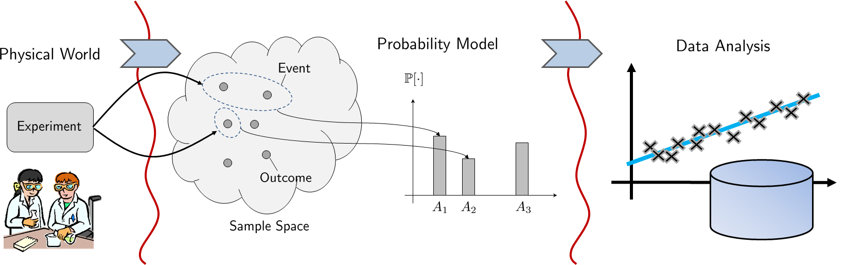
Therefore, whenever you talk about “probability,” you need to specify the triplet $(\Omega, \calF, \Pb)$ to define the probability space.

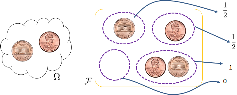
The necessity of the three elements is illustrated in Figure 2.12. The sample space is the interface with the physical world. It is the collection of all possible states that can result from an experiment. Some outcomes are more likely to happen, and some are less likely, but this does not matter because the sample space contains every possible outcome. The probability law is the interface with the data analysis. It is this law that defines the likelihood of each of the outcomes. However, since the probability law measures the size of a set, the probability law itself must be a function, a function whose argument is a set and whose value is a number. An outcome in the sample space is not a set. Instead, a subset in the sample space is a set. Therefore, the probability should input a subset and map it to a number. The collection of all possible subsets is the event space.

A perceptive reader like you may be wondering why we want to complicate things to this degree when calculating probability is trivial, e.g., throwing a die gives us a probability $\frac{1}{6}$ per face. In a simple world where problems are that easy, you can surely ignore all of these complications and proceed to the answer $\frac{1}{6}$. However, modern data analysis is not so easy. If we are given an image of size $64 \times 64$ pixels, how do we tell whether this image is of a cat or a dog? We need to construct a probability model that tells us the likelihood of having a particular $64 \times 64$ image. What should be included in this probability model? We need to know all the possible cases (the sample space), all the possible events (the event space), and the probability of each of the events (the probability law). If we know all of these, then our decision will be theoretically optimal. Of course, for high-dimensional data like images, we need approximations to such a probability model. However, we first need to understand the theoretical foundation of the probability space to know what approximations would make sense.

2.2.1Sample space $\Omega$

We start by defining the sample space $\Omega$. Given an experiment, the sample space $\Omega$ is the set containing all possible outcomes of the experiment.

Definition 2.13 (Sample Space)

A sample space $\Omega$ is the set of all possible outcomes from an experiment. We denote $\xi$ as an element in $\Omega$.

A sample space can contain discrete outcomes or continuous outcomes, as shown in the examples below and Figure 2.13.

Example 2.21

Example 2.21: (Discrete Outcomes)

sep0ex
Coin flip: $\Omega = \{H, \; T\}$.
Throw a die: $\Omega = \{\mydice{1}, \mydice{2}, \mydice{3}, \mydice{4}, \mydice{5}, \mydice{6}\}$.
Paper / scissor / stone: $\Omega = \{\text{paper}, \text{scissor}, \text{stone}\}$.
Draw an even integer: $\Omega = \{2,4,6,8,\ldots\}$.

Example 2.22

Example 2.22: (Continuous Outcomes)

sep0ex
Waiting time for a bus in West Lafayette: $\Omega = \{t \;\;|\;\; 0 \le t \le 30 \; \mathrm{ minutes}\}$.
Phase angle of a voltage: $\Omega = \{\theta \;\;|\;\; 0 \le \theta \le 2\pi\}$.
Frequency of a pitch: $\Omega = \{f \;\;|\;\; 0 \le f \le f_{\max}\}$.

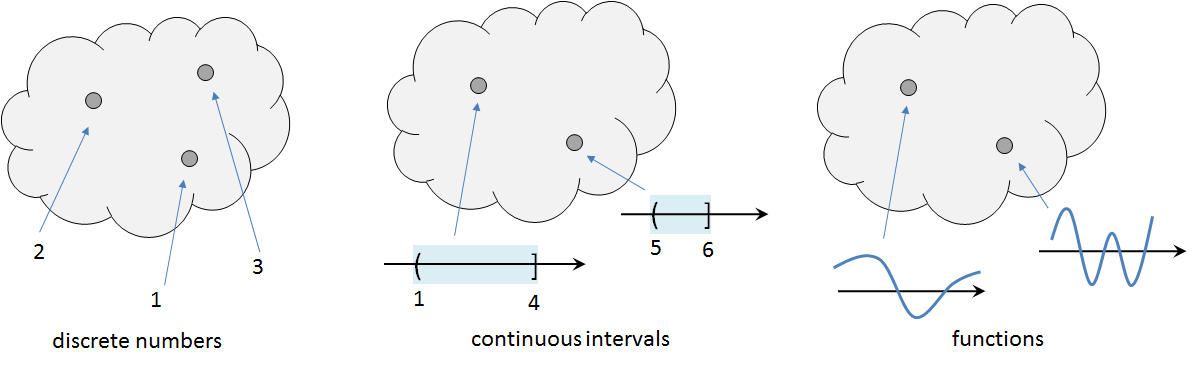
Figure 2.13 also shows a functional example of the sample space. In this case, the sample space contains functions. For example,

sep0ex
Set of all straight lines in 2D: $$\Omega = \{f \;|\; f(x) = ax + b, \; a, b \in \R\}.$$
Set of all cosine functions with a phase offset: $$\Omega = \{f \;|\; f(t) = \cos(2\pi\omega_0 t + \Theta), \; 0 \le \Theta \le 2\pi\}.$$

As we see from the above examples, the sample space is nothing but a universal set. The elements inside the sample space are the outcomes of the experiment. If you change the experiment, the possible outcomes will be different so that the sample space will be different. For example, flipping a coin has different possible outcomes from throwing a die.

What if we want to describe a composite experiment where we flip a coin and throw a die? Here is the sample space:

Example 2.23

Example 2.23: If the experiment contains flipping a coin and throwing a die, then the sample space is

\begin{aligned} \bigg\{&(H,\mydice{1}), (H,\mydice{2}), (H,\mydice{3}), (H,\mydice{4}), (H,\mydice{5}), (H,\mydice{6}), \\ &(T,\mydice{1}), (T,\mydice{2}), (T,\mydice{3}), (T,\mydice{4}), (T,\mydice{5}), (T,\mydice{6}) \bigg\}. \end{aligned}

In this sample space, each element is a pair of outcomes.

Practice Exercise 2.8

There are 8 processors on a computer. A computer job scheduler chooses one processor randomly. What is the sample space? If the computer job scheduler can choose two processors at once, what is the sample space then?

Solution

The sample space of the first case is $\Omega = \{1,2,3,4,5,6,7,8\}$. The sample space of the second case is $\Omega = \{(1,2), (1,3), (1,4), \ldots, (7,8)\}$.

Practice Exercise 2.9

A cell phone tower has a circular average coverage area of radius of 10 km. We observe the source locations of calls received by the tower. What is the sample space of all possible source locations?

Solution

Assume that the center of the tower is located at $(x_0,y_0)$. The sample space is the set $$\Omega = \{ (x,y) \;|\; \sqrt{(x-x_0)^2 + (y-y_0)^2} \le 10\}.$$

Not every set can be a sample space. A sample space must be exhaustive and exclusive. The term “exhaustive” means that the sample space has to cover all possible outcomes. If there is one possible outcome that is left out, then the set is no longer a sample space. The term “exclusive” means that the sample space contains unique elements so that there is no repetition of elements.

Example 2.24 (Counter examples)

The following two examples are NOT sample spaces.

sep0ex
Throw a die: $\Omega = \{1,2,3\}$ is not a sample space because it is not exhaustive.
Throw a die: $\Omega = \{1,1,2,3,4,5,6\}$ is not a sample space because it is not exclusive.

Therefore, a valid sample space must contain all possible outcomes, and each element must be unique.

We summarize the concept of a sample space as follows.

What is a sample space $\Omega$?

sep0ex
A sample space $\Omega$ is the collection of all possible outcomes.
The outcomes can be numbers, alphabets, vectors, or functions. The outcomes can also be images, videos, EEG signals, audio speeches, etc.
$\Omega$ must be exhaustive and exclusive.

2.2.2Event space $\calF$

The sample space contains all the possible outcomes. However, in many practical situations, we are not interested in each of the individual outcomes; we are interested in the combinations of the outcomes. For example, when throwing a die, we may ask “What is the probability of rolling an odd number?” or “What is the probability of rolling a number that is less than 3?” Clearly, “odd number” is not an outcome of the experiment because the possible outcomes are $\{\mydice{1}, \mydice{2}, \mydice{3}, \mydice{4}, \mydice{5}, \mydice{6}\}$. We call “odd number” an event. An event must be a subset in the sample space.

Definition 2.14 (Event)

An event $E$ is a subset in the sample space $\Omega$. The set of all possible events is denoted as $\calF$.

While this definition is extremely simple, we need to keep in mind a few facts about events. First, an outcome $\xi$ is an element in $\Omega$ but an event $E$ is a subset contained in $\Omega$, i.e., $E \subseteq \Omega$. Thus, an event can contain one outcome but it can also contain many outcomes. The following example shows a few cases of events:

Example 2.25

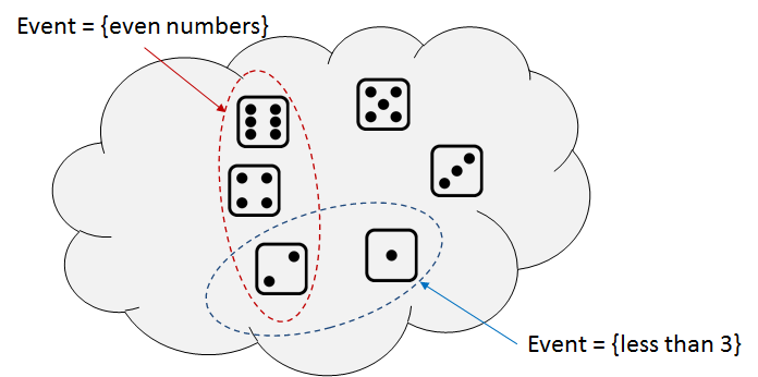
Throw a die. Let $\Omega = \{\mydice{1}, \mydice{2}, \mydice{3}, \mydice{4}, \mydice{5}, \mydice{6}\}$. The following are two possible events, as illustrated in Figure 2.14.

sep0ex
$E_1 = \{\mbox{even numbers}\} = \{ \mydice{2}, \mydice{4}, \mydice{6}\}$.
$E_2 = \{\mbox{less than 3}\} = \{\mydice{1}, \mydice{2}\}$.

Practice Exercise 2.10

The “ping” command is used to measure round-trip times for Internet packets. What is the sample space of all possible round-trip times? What is the event that a round-trip time is between 10 ms and 20 ms?

Solution

The sample space is $\Omega = [0,\infty)$. The event is $E = [10,20]$.

Practice Exercise 2.11

A cell phone tower has a circular average coverage area of radius 10 km. We observe the source locations of calls received by the tower. What is the event when the source location of a call is between 2 km and 5 km from the tower?

Solution

Assume that the center of the tower is located at $(x_0,y_0)$. The event is $E = \{ (x,y) \;|\; 2\le \sqrt{(x-x_0)^2 + (y-y_0)^2} \le 5\}$.

The second point we should remember is the cardinality of $\Omega$ and that of $\calF$. A sample space containing $n$ elements has a cardinality $n$. However, the event space constructed from $\Omega$ will contain $2^n$ events. To see why this is so, let's consider the following example.

Example 2.26

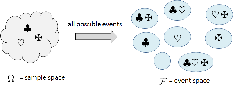
Consider an experiment with 3 outcomes $\Omega = \{\clubsuit,\heartsuit,\maltese\}$. We can list out all the possible events: $\emptyset$, $\{\clubsuit\}$, $\{\heartsuit\}$, $\{\maltese\}$, $\{\clubsuit,\heartsuit\}$, $\{\clubsuit,\maltese\}$, $\{\heartsuit,\maltese\}$, $\{\clubsuit,\heartsuit,\maltese\}$. So in total there are $2^3 = 8$ possible events. Figure 2.15 depicts the situation. What is the difference between $\clubsuit$ and $\{\clubsuit\}$? The former is an element, whereas the latter is a set. Thus, $\{\clubsuit\}$ is an event but $\clubsuit$ is not an event. Why is $\emptyset$ an event? Because we can ask “What is the probability that we get an odd number and an even number?” The probability is obviously zero, but the reason it is zero is that the event is an empty set.

**Figure 2.15.** The event space contains all the possible subsets inside the sample space.

In general, if there are $n$ elements in the sample space, then the number of events is $2^n$. To see why this is true, we can assign to each element a binary value: either 0 or 1. For example, in Table tab: ch2 event size dice we consider throwing a die. For each of the six faces, we assign a binary code. This will give us a binary string for each event. For example, the event $\{\mydice{1}, \mydice{5}\}$ is encoded as the binary string 100010 because only $\mydice{1}$ and $\mydice{5}$ are activated. We can count the total number of unique strings, which is the number of strings that can be constructed from $n$ bits. It is easily seen that this number is $2^n$.

Event	$\mydice{1}$	$\mydice{2}$	$\mydice{3}$	$\mydice{4}$	$\mydice{5}$	$\mydice{6}$	Binary Code
$\emptyset$	$\times$	$\times$	$\times$	$\times$	$\times$	$\times$	000000
$\{\mydice{1}, \mydice{5}\}$	$\bigcirc$	$\times$	$\times$	$\times$	$\bigcirc$	$\times$	100010
$\{\mydice{3}, \mydice{4}, \mydice{5}\}$	$\times$	$\times$	$\bigcirc$	$\bigcirc$	$\bigcirc$	$\times$	001110

$\{\mydice{2}, \mydice{3}, \mydice{4}, \mydice{5}, \mydice{6}\}$	$\times$	$\bigcirc$	$\bigcirc$	$\bigcirc$	$\bigcirc$	$\bigcirc$	011111
$\{\mydice{1}, \mydice{2}, \mydice{3}, \mydice{4}, \mydice{5}, \mydice{6}\}$	$\bigcirc$	$\bigcirc$	$\bigcirc$	$\bigcirc$	$\bigcirc$	$\bigcirc$	111111

Table 2.1. An event space contains $2^n$ events, where $n$ is the number of elements in the sample space. To see this, we encode each outcome with a binary code. The resulting binary string then forms a unique index of the event. Counting the total number of events gives us the cardinality of the event space.

The box below summarizes what you need to know about event spaces.

What is an event space $\calF$?

sep0ex
An event space $\calF$ is the set of all possible subsets. It is a set of sets.
We need $\calF$ because the probability law $\Pb$ is mapping a set to a number. $\Pb$ does not take an outcome from $\Omega$ but a subset inside $\Omega$.

Event spaces: Some advanced topics

The following discussions can be skipped if it is your first time reading the book.

What else do we need to take care of in order to ensure that an event is well defined? A few set operations seem to be necessary. For example, if $E_1 = \{\mydice{1}\}$ and $E_2 = \{\mydice{2}\}$ are events, it is necessary that $E = E_1 \cup E_2 = \{\mydice{1},\mydice{2}\}$ is an event too. Another example: if $E_1 = \{\mydice{5},\mydice{6}\}$ and $E_2 = \{\mydice{1},\mydice{5}\}$ are events, then it is necessary that $E = E_1 \cap E_2 = \{\mydice{5}\}$ is also an event. The third example: if $E_1 = \{\mydice{3},\mydice{4},\mydice{5},\mydice{6}\}$ is an event, then $E = E_1^c = \{\mydice{1},\mydice{2}\}$ should be an event. As you can see, there is nothing sophisticated in these examples. They are just some basic set operations. We want to ensure that the event space is closed under these set operations. That is, we do not want to be surprised by finding that a set constructed from two events is not an event. However, since all set operations can be constructed from union, intersection and complement, ensuring that the event space is closed under these three operations effectively ensures that it is closed to all set operations.

The formal way to guarantee these is the notion of a field. This term may seem to be abstract, but it is indeed quite useful:

Definition 2.15 (Field)

For an event space $\calF$ to be valid, $\calF$ must be a field $\calF$. It is a field if it satisfies the following conditions

sep0ex
$\emptyset \in \calF$ and $\Omega \in \calF$.
(Closed under complement) If $F \in \calF$, then also $F^c \in \calF$.
(Closed under union and intersection) If $F_1 \in \calF$ and $F_2 \in \calF$, then $F_1\cap F_2 \in \calF$ and $F_1 \cup F_2 \in \calF$.

For a finite set, i.e., a set that contains $n$ elements, the collection of all possible subsets is indeed a field. This is not difficult to see if you consider rolling a die. For example, if $E = \{\mydice{3},\mydice{4},\mydice{5},\mydice{6}\}$ is inside $\calF$, then $E^c = \{\mydice{1},\mydice{2}\}$ is also inside $\calF$. This is because $\calF$ consists of $2^n$ subsets each being encoded by a unique binary string. So if $E = 001111$, then $E^c = 110000$, which is also in $\calF$. Similar reasoning applies to intersection and union.

At this point, you may ask:

sep0ex
Why bother constructing a field? The answer is that probability is a measure of the size of a set, so we must input a set to a probability measure $\Pb$ to get a number. The set being input to $\Pb$ must be a subset inside the sample space; otherwise, it will be undefined. If we regard $\Pb$ as a mapping, we need to specify the collection of all its inputs, which is the set of all subsets, i.e., the event space. So if we do not define the field, there is no way to define the measure $\Pb$.
What if the event space is not a field? If the event space is not a field, then we can easily construct pathological cases where we cannot assign a probability. For example, if the event space is not a field, then it would be possible that the complement of $E = \{\mydice{3},\mydice{4},\mydice{5},\mydice{6}\}$ (which is $E^c = \{\mydice{1},\mydice{2}\}$) is not an event. This just does not make sense.

The concept of a field is sufficient for finite sample spaces. However, there are two other types of sample spaces where the concept of a field is inadequate. The first type of sets consists of the countably infinite sets, and the second type consists of the sets defined on the real line. There are other types of sets, but these two have important practical applications. Therefore, we need to have a basic understanding of these two types.

Sigma-field

The difficulty of a countably infinite set is that there are infinitely many subsets in the field of a countably infinite set. Having a finite union and a finite intersection is insufficient to ensure the closedness of all intersections and unions. In particular, having $F_1 \cup F_2 \in \calF$ does not automatically give us $\bigcup_{n=1}^{\infty} F_n \in \calF$ because the latter is an infinite union. Therefore, for countably infinite sets, their requirements to be a field are more restrictive as we need to ensure infinite intersection and union. The resulting field is called the $\sigma$-field.

Definition 2.16 ($\sigma$-field)

A sigma-field ($\sigma$-field) $\calF$ is a field such that

sep0ex
$\calF$ is a field, and
if $F_1,F_2,\ldots \in \calF$, then the union $\bigcup_{i=1}^{\infty}F_i$ and the intersection $\bigcap_{i=1}^{\infty}F_i$ are both in $\calF$.

When do we need a $\sigma$-field? When the sample space is countable and has infinitely many elements. For example, if the sample space contains all integers, then the collection of all possible subsets is a $\sigma$-field. For another, if $E_1 = \{2\}$, $E_2 = \{4\}$, $E_3 = \{6\}$, …, then $\bigcup_{n=1}^{\infty} E_n = \{2,4,6,8,~\ldots\} = \{\text{positive even numbers}\}$. Clearly, we want $\bigcup_{n=1}^{\infty} E_n$ to live in the sample space.

Borel sigma-field

While a sigma-field allows us to consider countable sets of events, it is still insufficient for considering events defined on the real line, e.g., time, as these events are not countable. So how do we define an event on the real line? It turns out that we need a different way to define the smallest unit. For finite sets and countable sets, the smallest units are the elements themselves because we can count them. For the real line, we cannot count the elements because any non-empty interval is uncountably infinite.

The smallest unit we use to construct a field for the real line is a semi-closed interval $$(-\infty, b] \bydef \{ x \;|\; -\infty < x \le b\}.$$ The Borel $\sigma$-field is defined as the sigma-field generated by the semi-closed intervals.

Definition 2.17 (Borel $\sigma$-field)

The Borel $\sigma$-field $\calB$ is a $\sigma$-field generated from semi-closed intervals: $$(-\infty, b] \bydef \{ x \;|\; -\infty < x \le b\}.$$

The difference between the Borel $\sigma$-field $\calB$ and a regular $\sigma$-field is how we measure the subsets. In a $\sigma$-field, we count the elements in the subsets, whereas, in a Borel $\sigma$-field, we use the semi-closed intervals to measure the subsets.

Being a field, the Borel $\sigma$-field is closed under complement, union, and intersection. In particular, subsets of the following forms are also in the Borel $\sigma$-field $\calB$: $$(a,b), \; [a,b], \; (a,b], \; [a,b), \; [a, \infty), \; (a,\infty), \; (-\infty, b], \; \{b\}.$$ For example, $(a,\infty)$ can be constructed from $(-\infty,a]^c$, and $(a,b]$ can be constructed by taking the intersection of $(-\infty,b]$ and $(a, \infty)$.

Example 2.27

Example 2.27: Waiting for a bus. Let $\Omega = \{0 \le t \le 30\}$. The Borel $\sigma$-field contains all semi-closed intervals $(a,b]$, where $0 \le a \le b \le 30$. Here are two possible events:

sep0em
$F_1 = \{\mbox{less than 10 minutes}\} = \{ 0 \le t < 10\} = \{0\} \cup (\{0 < t \le 10\} \cap \{10\}^c)$.
$F_2 = \{\mbox{more than 20 minutes}\} = \{ 20 < t \le 30\}$.

Further discussion of the Borel $\sigma$-field can be found in Leon-Garcia (3rd Edition), Chapter 2.9.

This is the end of the discussion. Please join us again.

2.2.3Probability law $\Pb$

The third component of a probability space is the probability law $\Pb$. Its job is to assign a number to an event.

Definition 2.18 (Probability Law)

A probability law is a function $\Pb: \calF \rightarrow [0,1]$ of an event $E$ to a real number in $[0,\,1]$.

The probability law is thus a function, and therefore we must specify the input and the output. The input to $\Pb$ is an event $E$, which is a subset in $\Omega$ and an element in $\calF$. The output of $\Pb$ is a number between 0 and 1, which we call the probability.

The definition above does not specify how an event is being mapped to a number. However, since probability is a measure of the size of a set, a meaningful $\Pb$ should be consistent for all events in $\calF$. This requires some rules, known as the axioms of probability, when we define the $\Pb$. Any probability law $\Pb$ must satisfy these axioms; otherwise, we will see contradictions. We will discuss the axioms in the next section. For now, let us look at two examples to make sure we understand the functional nature of $\Pb$.

Example 2.28

Consider flipping a coin. The event space is $\calF = \{ \emptyset, \{H\}, \{T\}, \Omega\}$. We can define the probability law as $$\Pb[\emptyset] = 0,\;\; \Pb[\{H\}] = \frac12,\;\; \Pb[\{T\}] = \frac12,\;\; \Pb[\Omega] = 1,$$ as shown in Figure 2.16. This $\Pb$ is clearly consistent for all the events in $\calF$.

Is it possible to construct an invalid $\Pb$? Certainly. Consider the following probability law: $$\Pb[\emptyset] = 0,\;\; \Pb[\{H\}] = \frac13,\;\; \Pb[\{T\}] = \frac13,\;\; \Pb[\Omega] = 1.$$ This law is invalid because the individual events are $\Pb[\{H\}] = \frac13$ and $\Pb[\{T\}] = \frac13$ but the union is $\Pb[\Omega] = 1$. To fix this problem, one possible solution is to define the probability law as $$\Pb[\emptyset] = 0,\;\; \Pb[\{H\}] = \frac13,\;\; \Pb[\{T\}] = \frac23,\;\; \Pb[\Omega] = 1.$$ Then, the probabilities for all the events are well defined and consistent.

**Figure 2.16.** A probability law is a mapping from an event to a number. A probability law cannot be arbitrarily assigned; it must satisfy the axioms of probability.

Example 2.29

Example 2.29. Consider a sample space containing three elements $\Omega = \{\clubsuit,\heartsuit,\maltese\}$. The event space is then $\calF = \bigg\{\emptyset, \{\clubsuit\}, \{\heartsuit\}, \{\maltese\}, \{\clubsuit,\heartsuit\}, \{\heartsuit,\maltese\}, \{\clubsuit,\maltese\}, \{\clubsuit,\heartsuit,\maltese\}\bigg\}.$ One possible $\Pb$ we could define would be

\begin{aligned} &\Pb[\emptyset] = 0, \quad \Pb[\{\clubsuit\}]=\Pb[\{\heartsuit\}]=\Pb[\{\maltese\}]= \frac{1}{3},\\ &\Pb[\{\clubsuit,\heartsuit\}]=\Pb[\{\clubsuit,\maltese\}]=\Pb[\{\heartsuit,\maltese\}]= \frac{2}{3}, \quad \Pb[\{\clubsuit,\heartsuit,\maltese\}] = 1. \end{aligned}

What is a probability law $\Pb$?

sep0ex
A probability law $\Pb$ is a function.
It takes a subset (an element in $\calF$) and maps it to a number between 0 and 1.
$\Pb$ is a measure of the size of a set.
For $\Pb$ to be valid, it must satisfy the axioms of probability.

A probability law $\Pb$ is a measure

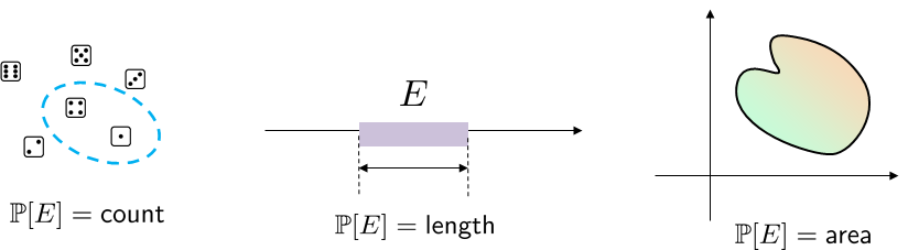
Consider the word “measure” in our slogan: probability is a measure of the size of a set. Depending on the nature of the set, the measure can be a counter, ruler, scale, or even a stopwatch. So far, all the examples we have seen are based on sets with a finite number of elements. For these sets, the natural choice of the probability measure is a counter. However, if the sets are intervals on the real line or regions in a plane, we need a different probability law to measure their size. Let's look at the examples shown in Figure 2.17.

Example 2.30

Example 2.30 (Finite Set). Consider throwing a die, so that $$\Omega = \{\mydice{1},\mydice{2},\mydice{3},\mydice{4},\mydice{5},\mydice{6}\}.$$ Then the probability measure is a counter that reports the number of elements. If the die is fair, i.e., all the 6 faces have equal probability of happening, then an event $E = \{\mydice{1},\mydice{3}\}$ will have a probability $\Pb[E] = \frac{2}{6}$.

Example 2.31

Example 2.31 (Intervals). Suppose that the sample space is a unit interval $\Omega = [0,1]$. Let $E$ be an event such that $E = [a,b]$ where $a,b$ are numbers in $[0,1]$. Then the probability measure is a ruler that measures the length of the intervals. If all the numbers on the real line have equal probability of appearing, then $\Pb[E] = b-a$.

Example 2.32

Example 2.32 (Regions). Suppose that the sample space is the square $\Omega = [-1,1] \times [-1,1]$. Let $E$ be a circle such that $E = \{(x,y)| x^2+y^2 < r^2\}$, where $r < 1$. Then the probability measure is an area measure that returns us the area of $E$. If we assume that all coordinates in $\Omega$ are equally probable, then $\Pb[E] = \dfrac{\pi r^2}{4}$, for $r < 1$.

**Figure 2.17.** Probability is a measure of the size of a set. The probability can be a counter that counts the number of elements, a ruler that measures the length of an interval, or an integration that measures the area of a region.

Because probability is a measure of the size of a set, two sets can be compared according to their probability measures. For example, if $\Omega = \{\clubsuit,\heartsuit,\maltese\}$, and if $E_1 = \{\clubsuit\}$ and $E_2= \{\clubsuit,\heartsuit\}$, then one possible $\Pb$ is to assign $\Pb[E_1] = \Pb[\{\clubsuit\}] = \frac13$ and $\Pb[E_2] = \Pb[\{\clubsuit,\heartsuit\}] = 2/3$. In this particular case, we see that $E_1 \subseteq E_2$ and thus $$\Pb[E_1] \le \Pb[E_2].$$

Let's now consider the term “size.” Notice that the concept of the size of a set is not limited to the number of elements. A better way to think about size is to imagine that it is the weight of the set. This may seem fanciful at first, but it is quite natural. Consider the following example.

Example 2.33

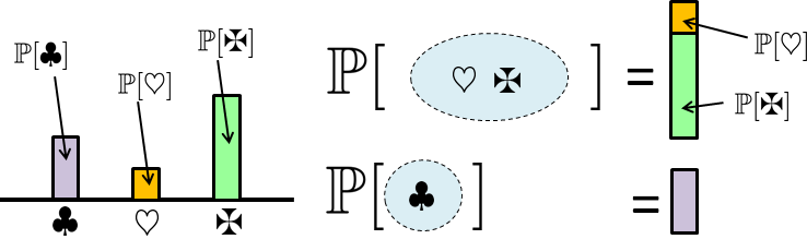
(Discrete events with different weights) Suppose we have a sample space $\Omega = \{\clubsuit,\heartsuit,\maltese\}$. Let us assign a different probability to each outcome:

\begin{aligned} \Pb[\{\clubsuit\}] = \frac{2}{6}, \quad \Pb[\{\heartsuit\}] = \frac{1}{6}, \quad \Pb[\{\maltese\}] = \frac{3}{6}. \end{aligned}

As illustrated in Figure 2.18, since each outcome has a different weight, when determining the probability of a set of outcomes we can add these weights (instead of counting the number of outcomes). For example, when reporting $\Pb[\{\clubsuit\}]$ we find its weight $\Pb[\{\clubsuit\}] = \frac26$, whereas when reporting $\Pb[\{\heartsuit,\maltese\}]$ we find the sum of their weights $\Pb[\{\heartsuit,\maltese\}] = \frac16+\frac36 = \frac46$. Therefore, the notion of size does not refer to the number of elements but to the total weight of these elements.

Example 2.34

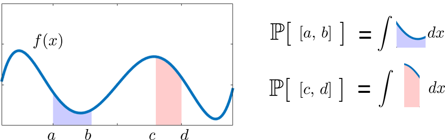
Example 2.34. (Continuous events with different weights) Suppose that the sample space is an interval, say $\Omega = [-1,1]$. On this interval we define a weighting function $f(x)$ where $f(x_0)$ specifies the weight for $x_0$. Because $\Omega$ is an interval, events defined on this $\Omega$ must also be intervals. For example, we can consider two events $E_1 = [a,b]$ and $E_2 = [c,d]$. The probabilities of these events are $\Pb[E_1] = \int_a^b f(x) \;dx$ and $\Pb[E_2] = \int_c^d f(x) \;dx$, as shown in Figure 2.19.

**Figure 2.19.** If the sample space is an interval on the real line, then the probability of an event is the area under the curve of the weighting function.

Viewing probability as a measure is not just a game for mathematicians; rather, it has fundamental significance for several reasons. First, it eliminates any dependency on probability as relative frequency from the frequentist point of view. Relative frequency is a narrowly defined concept that is largely limited to discrete events, e.g., flipping a coin. While we can assign weights to coin-toss events to deal with those biased coins, the extension to continuous events becomes problematic. By thinking of probability as a measure, we can generalize the notion to apply to intervals, areas, volumes, and so on.

Second, viewing probability as a measure forces us to disentangle an event from measures. An event is a subset in the sample space. It has nothing to do with the measure (e.g., a ruler) you use to measure the event. The measure, on the other hand, specifies the weighting function you apply to measure the event when computing the probability. For example, let $\Omega = [-1,1]$ be an interval, and let $E = [a,b]$ be an event. We can define two weighting functions $f(x)$ and $g(x)$. Correspondingly, we will have two different probability measures $\mathbb{F}$ and $\mathbb{G}$ such that

\begin{aligned} \mathbb{F}([a,b]) &= \int_{E} d\mathbb{F} = \int_{a}^{b} f(x) \;dx, \\ \mathbb{G}([a,b]) &= \int_{E} d\mathbb{G} = \int_{a}^{b} g(x) \;dx. \end{aligned}

To make sense of these notations, consider only $\Pb[[a,b]]$ and not $\mathbb{F}([a,b])$ and $\mathbb{G}([a,b])$. As you can see, the event for both measures is $E = [a,b]$ but the measures are different. Therefore, the values of the probability are different.

Example 2.35

(Two probability laws are different if their weighting functions are different.) Consider two different weighting functions for throwing a die. The first one assigns probability as the following:

\begin{aligned} \Pb[\{\mydice{1}\}] &= \frac{1}{12}, \; \Pb[\{\mydice{2}\}] = \frac{2}{12}, \; \Pb[\{\mydice{3}\}] = \frac{3}{12}, \\ \; \Pb[\{\mydice{4}\}] &= \frac{4}{12}, \; \Pb[\{\mydice{5}\}] = \frac{1}{12}, \; \Pb[\{\mydice{6}\}] = \frac{1}{12}, \end{aligned}

whereas the second function assigns the probability like this:

\begin{aligned} \Pb[\{\mydice{1}\}] &= \frac{2}{12}, \; \Pb[\{\mydice{2}\}] = \frac{2}{12}, \; \Pb[\{\mydice{3}\}] = \frac{2}{12},\\ \; \Pb[\{\mydice{4}\}] &= \frac{2}{12}, \; \Pb[\{\mydice{5}\}] = \frac{2}{12}, \; \Pb[\{\mydice{6}\}] = \frac{2}{12}. \end{aligned}

Let an event $E = \{\mydice{1},\mydice{2}\}$. Let $\mathbb{F}$ be the measure using the first set of probabilities, and let $\mathbb{G}$ be the measure of the second set of probabilities. Then,

\begin{aligned} \mathbb{F}(E) &= \mathbb{F}(\{\mydice{1},\mydice{2}\}) = \frac{1}{12} + \frac{2}{12} = \frac{3}{12},\\ \mathbb{G}(E) &= \mathbb{G}(\{\mydice{1},\mydice{2}\}) = \frac{2}{12} + \frac{2}{12} = \frac{4}{12}. \end{aligned}

Therefore, although the events are the same, the two different measures will give us two different probability values.

Remark. The notation $\int_{E} d\mathbb{F}$ in Eq. (2.20) is known as the Lebesgue integral. You should be aware of this notation, but the theory of Lebesgue measure is beyond the scope of this book.

2.2.4Measure zero sets

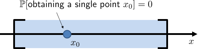
Understanding the measure perspective on probability allows us to understand another important concept of probability, namely measure zero sets. To introduce this concept, we pose the question: What is the probability of obtaining a single point, say $\{0.5\}$, when the sample space is $\Omega = [0,1]$?

The answer to this question is rooted in the compatibility between the measure and the sample space. In other words, the measure has to be meaningful for the events in the sample space. Using $\Omega = [0,1]$, since $\Omega$ is an interval, an appropriate measure would be the length of this interval. You may add different weighting functions to define your measure, but ultimately, the measure must be an integral. If you use a “counter” as a measure, then the counter and the interval are not compatible because you cannot count on the real line.

Now, suppose that we define a measure for $\Omega = [0,1]$ using a weighting function $f(x)$. This measure is determined by an integration. Then, for $E = \{0.5\}$, the measure is

\Pb[E] = \Pb[\{0.5\}] = \int_{0.5}^{0.5} f(x) \;dx = 0.

In fact, for any weighting function the integral will be zero because the length of the set $E$ is zero. (We assume that $f$ is continuous throughout $[0,1]$. If $f$ is discontinuous at $x = 0.5$, some additional considerations will apply. ) An event that gives us zero probability is known as an event with measure 0. Figure 2.20 shows an example.

**Figure 2.20.** The probability of obtaining a single point in a continuous interval is zero.

What are measure zero sets?

sep0ex
A set $E$ (non-empty) is called a measure zero set when $\Pb[E] = 0$.
For example, $\{0\}$ is a measure zero set when we use a continuous measure $\mathbb{F}$.
But $\{0\}$ can have a positive measure when we use a discrete measure $\mathbb{G}$.

Example 2.36

Example 2.36(a). Consider a fair die with $\Omega = \{\mydice{1},\mydice{2},\mydice{3},\mydice{4},\mydice{5},\mydice{6}\}$. Then the set $\{\mydice{1}\}$ has a probability of $\frac{1}{6}$. The sample space does not have a measure zero event because the measure we use is a counter.

Example 2.36(b). Consider an interval with $\Omega = [1,6]$. Then the set $\{1\}$ has measure 0 because it is an isolated point with respect to the sample space.

Example 2.36(c). For any intervals, $\Pb[[a,b]] = \Pb[(a,b)]$ because the two end points have measure zero: $\Pb[\{a\}] = \Pb[\{b\}] = 0$.

Formal definitions of measure zero sets

The following discussion of the formal definitions of measure zero sets is optional for the first reading of this book.

We can formally define measure zero sets as follows:

Definition 2.19 (Measure Zero)

Let $\Omega$ be the sample space. A set $A \subseteq \Omega$ is said to have measure zero if for any given $\epsilon > 0$,

sep0ex
There exists a countable number of subsets $A_n$ such that $A \subseteq \cup_{n=1}^\infty A_n$, and
$\sum_{n=1}^\infty \Pb[A_n] < \epsilon$.

You may need to read this definition carefully. Suppose we have an event $A$. We construct a set of neighbors $A_1,\ldots,A_{\infty}$ such that $A$ is included in the union $\cup_{n=1}^\infty A_n$. If the sum of all $\Pb[A_n]$ is still less than $\epsilon$, then the set $A$ will have a measure zero.

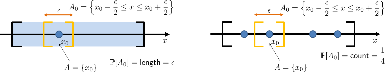
To understand the difference between a measure for a continuous set and a countable set, consider Figure 2.21. On the left side of Figure 2.21 we show an interval $\Omega$ in which there is an isolated point $x_0$. The measure for this $\Omega$ is the length of the interval (relative to whatever weighting function you use). We define a small neighborhood $A_0 = (x_0-\frac{\epsilon}{2}, \; x_0+\frac{\epsilon}{2})$ surrounding $x_0$. The length of this interval is not more than $\epsilon$. We then shrink $\epsilon$. However, regardless of how small $\epsilon$ is, since $x_0$ is an isolated point, it is always included in the neighborhood. Therefore, the definition is satisfied, and so $\{x_0\}$ has measure zero.

Example 2.37

Let $\Omega = [0,1]$. The set $\{0.5\} \subset \Omega$ has measure zero, i.e., $\Pb[\{0.5\}] = 0$. To see this, we draw a small interval around 0.5, say $[0.5-\epsilon/3, 0.5+\epsilon/3]$. Inside this interval, there is really nothing to measure besides the point 0.5. Thus we have found an interval such that it contains 0.5, and the probability is $\Pb[[0.5-\epsilon/3, 0.5+\epsilon/3]] = 2\epsilon/3 < \epsilon$. Therefore, by definition, the set $\{0.5\}$ has measure 0.

The situation is very different for the right-hand side of Figure 2.21. Here, the measure is not the length but a counter. So if we create a neighborhood surrounding the isolated point $x_0$, we can always make a count. As a result, if you shrink $\epsilon$ to become a very small number (in this case less than $\frac{1}{4}$), then $\Pb[\{x_0\}] < \epsilon$ will no longer be true. Therefore, the set $\{x_0\}$ has a non-zero measure when we use the counter as the measure.

When we make probabilistic claims without considering the measure zero sets, we say that an event happens almost surely.

Definition 2.20 (Almost Surely)

An event $A \subseteq \R$ is said to hold almost surely (a.s.) if

\Pb[A] = 1

except for all measure zero sets in $\R$.

Therefore, if a set $A$ contains measure zero subsets, we can simply ignore them because they do not affect the probability of events. In this book, we will omit “a.s.” if the context is clear.

Example 2.38

Example 2.38(a). Let $\Omega = [0,1]$. Then $\Pb[(0,1)] = 1$ almost surely because the points 0 and 1 have measure zero in $\Omega$.

Example 2.38(b). Let $\Omega = \{x \;|\; x^2 \le 1\}$ and let $A = \{x \;|\; x^2 < 1\}$. Then $\Pb[A] = 1$ almost surely because the circumference has measure zero in $\Omega$.

Practice Exercise 2.12

Let $\Omega = \{f : \R \rightarrow [-1,1] \,|\, f(t) = \cos(\omega_0 t + \theta)\}$, where $\omega_0$ is a fixed constant and $\theta$ is random. Construct a measure zero event and an almost sure event.

Solution

Let $$E = \{f : \R \rightarrow [-1,1] \,|\, f(t) = \cos(\omega_0 t + k \pi/2)\}$$ for any integer $k$. That is, $E$ contains all the functions with a phase of $\pi/2$, $2\pi/2$, $3\pi/2$, etc. Then $E$ will have measure zero because it is a countable set of isolated functions. The event $E^c$ will have probability $\Pb[E^c] = 1$ almost surely because $E$ has measure zero.

This is the end of the discussion. Please join us again.

2.2.5Summary of the probability space

Let's try to understand our slogan: probability is a measure of the size of a set. This slogan is precise, but it needs clarification. When we say probability is a measure, we are thinking of it as being the probability law $\Pb$. Of course, in practice, we always think of probability as the number returned by the measure. However, the difference is not crucial. Also, “size” not only means the number of elements in the set, but it also means the relative weight of the set in the sample space. For example, if we use a weight function to weigh the set elements, then size would refer to the overall weight of the set.

When we put all of these pieces together, we can understand why a probability space must consist of the three components

(\Omega, \calF, \Pb),

where $\Omega$ is the sample space that defines all possible outcomes, $\calF$ is the event space generated from $\Omega$, and $\Pb$ is the probability law that maps an event to a number in $[0,1]$. Can we drop one or more of the three components? We cannot! If we do not specify the sample space $\Omega$, then there is no way to define the events. If we do not have a complete event space $\calF$, then some events will become undefined, and further, if the probability law is applied only to outcomes, we will not be able to define the probability for events. Finally, if we do not specify the probability law, then we do not have a way to assign probabilities.

Event	\(\mydice{1}\)	\(\mydice{2}\)	\(\mydice{3}\)	\(\mydice{4}\)	\(\mydice{5}\)	\(\mydice{6}\)	Binary Code
\(\emptyset\)	\(\times\)	\(\times\)	\(\times\)	\(\times\)	\(\times\)	\(\times\)	000000
\(\{\mydice{1}, \mydice{5}\}\)	\(\bigcirc\)	\(\times\)	\(\times\)	\(\times\)	\(\bigcirc\)	\(\times\)	100010
\(\{\mydice{3}, \mydice{4}, \mydice{5}\}\)	\(\times\)	\(\times\)	\(\bigcirc\)	\(\bigcirc\)	\(\bigcirc\)	\(\times\)	001110

\(\{\mydice{2}, \mydice{3}, \mydice{4}, \mydice{5}, \mydice{6}\}\)	\(\times\)	\(\bigcirc\)	\(\bigcirc\)	\(\bigcirc\)	\(\bigcirc\)	\(\bigcirc\)	011111
\(\{\mydice{1}, \mydice{2}, \mydice{3}, \mydice{4}, \mydice{5}, \mydice{6}\}\)	\(\bigcirc\)	\(\bigcirc\)	\(\bigcirc\)	\(\bigcirc\)	\(\bigcirc\)	\(\bigcirc\)	111111

Probability Space

2.2.1Sample space \(\Omega\)

2.2.2Event space \(\calF\)

Event spaces: Some advanced topics

Sigma-field

Borel sigma-field

2.2.3Probability law \(\Pb\)

A probability law \(\Pb\) is a measure

2.2.4Measure zero sets

Formal definitions of measure zero sets

2.2.5Summary of the probability space