eBook › Chapter 2 · Probability

Section 2.4

Conditional Probability

In many practical data science problems, we are interested in the relationship between two or more events. For example, an event $A$ may cause $B$ to happen, and $B$ may cause $C$ to happen. A legitimate question in probability is then: If $A$ has happened, what is the probability that $B$ also happens? Of course, if $A$ and $B$ are correlated events, then knowing one event can tell us something about the other event. If the two events have no relationship, knowing one event will not tell us anything about the other.

In this section, we study the concept of conditional probability. There are three sub-topics in this section. We summarize the key points below.

The three main messages of this section are:

sep0ex
Section sec: ch2 conditional probability: Conditional probability. Conditional probability of $A$ given $B$ is $\Pb[A|B] = \frac{\Pb[A \cap B]}{\Pb[B]}$.
Section sec: ch2 independence: Independence. Two events are independent if the occurrence of one does not influence the occurrence of the other: $\Pb[A|B] = \Pb[A]$.
Section sec: ch2 Bayes: Bayes' theorem and the law of total probability. Bayes' theorem allows us to switch the order of the conditioning: $\Pb[A|B]$ vs. $\Pb[B|A]$, whereas the law of total probability allows us to decompose an event into smaller events.

2.4.1Definition of conditional probability

We start by defining conditional probability.

Definition 2.22 (Conditional Probability)

Consider two events $A$ and $B$. Assume $\Pb[B] \not= 0$. The conditional probability of $A$ given $B$ is

\Pb[A \,|\, B] \bydef \frac{\Pb[A \cap B]}{\Pb[B]}.

According to this definition, the conditional probability of $A$ given $B$ is the ratio of $\Pb[A \cap B]$ to $\Pb[B]$. It is the probability that $A$ happens when we know that $B$ has already happened. Since $B$ has already happened, the event that $A$ has also happened is represented by $A\cap B$. However, since we are only interested in the relative probability of $A$ with respect to $B$, we need to normalize using $B$. This can be seen by comparing $\Pb[A \,|\, B]$ and $\Pb[A \cap B]$:

\Pb[A \,|\, B] = \frac{\Pb[A \cap B]}{\Pb[B]} \quad\mbox{and}\quad \Pb[A \cap B] = \frac{\Pb[A \cap B]}{\Pb[\Omega]}.

The difference is illustrated in Figure 2.26: The intersection $\Pb[A \cap B]$ calculates the overlapping area of the two events. We make no assumptions about the cause-effect relationship.

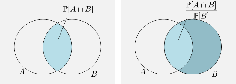
What justifies this ratio? Suppose that $B$ has already happened. Then, anything outside $B$ will immediately become irrelevant as far as the relationship between $A$ and $B$ is concerned. So when we ask: “What is the probability that $A$ happens given that $B$ has happened?”, we are effectively asking for the probability that $A \cap B$ happens under the condition that $B$ has happened. Note that we need to consider $A \cap B$ because we know that $B$ has already happened. If we take $A$ only, then there exists a region $A \backslash B$ which does not contain anything about $B$. However, since we know that $B$ has happened, $A \backslash B$ is impossible. In other words, among the elements of $A$, only those that appear in $A \cap B$ are meaningful.

Example 2.43

Let

\begin{aligned} A &= \{\mbox{Purdue gets Big Ten championship}\}, \\ B &= \{\mbox{Purdue wins 15 games consecutively}\}. \end{aligned}

In this example,

\begin{aligned} \Pb[A] &= \mbox{Prob. that Purdue gets the championship},\\ \Pb[B] &= \mbox{Prob. that Purdue wins 15 games consecutively},\\ \Pb[A \cap B] &= \mbox{Prob. that Purdue gets the championship and wins 15 games},\\ \Pb[A \,|\, B] &= \mbox{Prob. that Purdue gets the championship given that }\\ &\quad\;\; \mbox{Purdue won 15 games}. \end{aligned}

Without any additional information, it is unlikely that Purdue will get the championship because the sample space of all possible competition results is large. However, if we have already won 15 games consecutively, then the denominator of the probability becomes much smaller. In this case, the conditional probability is high.

Example 2.44

Consider throwing a die. Let

A = \{\mbox{getting a 3}\} \quad\mbox{and}\quad B = \{\mbox{getting an odd number}\}.

Find $\Pb[A \,|\, B]$ and $\Pb[B \,|\, A]$.

Solution

The following probabilities are easy to calculate:

\begin{aligned} \Pb[A] = \Pb[\{\mydice{3}\}] = \frac16, \qquad\mbox{and}\qquad \Pb[B] = \Pb[\{\mydice{1},\mydice{3},\mydice{5}\}] = \frac{3}{6}. \end{aligned}

Also, the intersection is

\begin{aligned} \Pb[A \cap B] = \Pb[\{\mydice{3}\}] = \frac{1}{6}. \end{aligned}

Given these values, the conditional probability of $A$ given $B$ can be calculated as

\begin{aligned} \Pb[A \,|\, B] = \frac{\Pb[A \cap B]}{\Pb[B]} = \frac{\frac{1}{6}}{\frac{3}{6}} = \frac{1}{3}. \end{aligned}

In other words, if we know that we have an odd number, then the probability of obtaining a 3 has to be computed over $\{\mydice{1},\mydice{3},\mydice{5}\}$, which give us a probability $\frac{1}{3}$. If we do not know that we have an odd number, then the probability of obtaining a 3 has to be computed from the sample space $\{\mydice{1},\mydice{2},\mydice{3},\mydice{4},\mydice{5},\mydice{6}\}$, which will give us $\frac{1}{6}$.

The other conditional probability is

\begin{aligned} \Pb[B \,|\, A] = \frac{\Pb[A \cap B]}{\Pb[A]} = 1. \end{aligned}

Therefore, if we know that we have rolled a 3, then the probability for this number being an odd number is 1.

Example 2.45

Consider the situation shown in Figure 2.27. There are 12 points with equal probabilities of happening. Find the probabilities $\Pb[A|B]$ and $\Pb[B|A]$.

Solution

In this example, we can first calculate the individual probabilities:

\begin{aligned} \Pb[A] = \frac{5}{12}, \quad\mbox{and}\quad \Pb[B] = \frac{6}{12}, \quad\mbox{and}\quad \Pb[A \cap B] = \frac{2}{12}. \end{aligned}

Then the conditional probabilities are

\begin{aligned} \Pb[A|B] &= \frac{\Pb[A \cap B]}{\Pb[B]} = \frac{\frac{2}{12}}{\frac{6}{12}} = \frac{1}{3},\\ \Pb[B|A] &= \frac{\Pb[A\cap B]}{\Pb[A]} = \frac{\frac{2}{12}}{\frac{5}{12}} = \frac{2}{5}. \end{aligned}

**Figure 2.27.** [Left] All the sets. [Middle] $\Pb[A|B]$ is the ratio between dots inside the light yellow region over those in yellow, which is $\frac{2}{6}$. [Right] $\Pb[B|A]$ is the ratio between dots inside the light pink region over those in pink, which is $\frac{2}{5}$.

Example 2.46

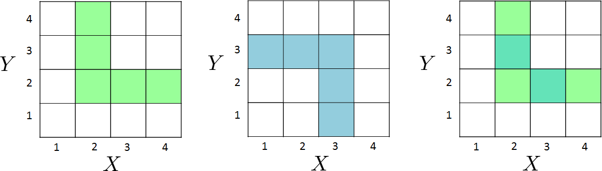
Consider a tetrahedral (4-sided) die. Let $X$ be the first roll and $Y$ be the second roll. Let $B$ be the event that $\min(X,Y) = 2$ and $M$ be the event that $\max(X,Y) = 3$. Find $\Pb[M | B]$.

Solution

As shown in Figure 2.28, the event $B$ is highlighted in green. (Why?) Similarly, the event $M$ is highlighted in blue. (Again, why?) Therefore, the probability is $$\Pb[M | B] = \frac{\Pb[M \cap B]}{\Pb[B]} = \frac{\frac{2}{16}}{\frac{5}{16}} = \frac{2}{5}.$$

Remark. Notice that if $\Pb[B] \le \Pb[\Omega]$, then $\Pb[A \,|\, B]$ is always larger than or equal to $\Pb[A \cap B]$, i.e.,

\Pb[A | B] \ge \Pb[A \cap B].

Conditional probabilities are legitimate probabilities

Conditional probabilities are legitimate probabilities. Given $B$, the probability $\Pb[A|B]$ satisfies Axioms I, II, III.

Theorem 2.6

Let $\Pb[B] > 0$. The conditional probability $\Pb[A \,|\, B]$ satisfies Axioms I, II, and III.

Proof. Let's check the axioms:

sep0ex
Axiom I: We want to show $$\Pb[A \,|\, B] = \frac{\Pb[A \cap B]}{\Pb[B]} \ge 0.$$ Since $\Pb[B] > 0$ and Axiom I requires $\Pb[A \cap B] \ge 0$, we therefore have $\Pb[A \,|\, B] \ge 0$.
Axiom II:
$\begin{aligned} \Pb[\Omega \,|\, B] &= \frac{\Pb[\Omega \cap B]}{\Pb[B]} \\ &= \frac{\Pb[B]}{\Pb[B]} = 1. \end{aligned}$
Axiom III: Consider two disjoint sets $A$ and $C$. Then,
$\begin{aligned} \Pb[A \cup C \,|\, B] &= \frac{\Pb[(A \cup C) \cap B]}{\Pb[B]} \\ &= \frac{\Pb[(A \cap B) \cup (C \cap B)]}{\Pb[B]}\\ &\overset{(a)}{=} \frac{\Pb[A \cap B]}{\Pb[B]} + \frac{\Pb[C \cap B]}{\Pb[B]} \\ &= \Pb[A|B] + \Pb[C|B], \end{aligned}$
where $(a)$ holds because if $A$ and $C$ are disjoint then $(A \cap B)\cap (C \cap B) = \emptyset$.

■

To summarize this subsection, we highlight the essence of conditional probability.

What are conditional probabilities?

sep0ex
Conditional probability of $A$ given $B$ is the ratio $\frac{\Pb[A \cap B]}{\Pb[B]}$.
It is again a measure. It measures the relative size of $A$ inside $B$.
Because it is a measure, it must satisfy the three axioms.

2.4.2Independence

Conditional probability deals with situations where two events $A$ and $B$ are related. What if the two events are unrelated? In probability, we have a technical term for this situation: statistical independence.

Definition 2.23 (Independence)

Two events $A$ and $B$ are statistically independent if

\Pb[A \cap B] = \Pb[A]\Pb[B].

Why define independence in this way? Recall that $\Pb[A \,|\, B] = \frac{\Pb[A \cap B]}{\Pb[B]}$. If $A$ and $B$ are independent, then $\Pb[A \cap B] = \Pb[A]\,\Pb[B]$ and so

\Pb[A \,|\, B] = \frac{\Pb[A \cap B]}{\Pb[B]} = \frac{\Pb[A] \; \Pb[B]}{\Pb[B]} = \Pb[A].

This suggests an interpretation of independence: If the occurrence of $B$ provides no additional information about the occurrence of $A$, then $A$ and $B$ are independent.

Therefore, we can define independence via conditional probability:

Definition 2.24 (Independence (via Conditional Probability))

Let $A$ and $B$ be two events such that $\Pb[A] > 0$ and $\Pb[B] > 0$. Then $A$ and $B$ are independent if

\Pb[A \,|\, B] = \Pb[A] \quad\mbox{or}\quad \Pb[B \,|\, A] = \Pb[B].

The two statements are equivalent as long as $\Pb[A] > 0$ and $\Pb[B] > 0$. This is because $\Pb[A|B] = \Pb[A\cap B]/\Pb[B]$. If $\Pb[A|B] = \Pb[A]$ then $\Pb[A\cap B] = \Pb[A]\Pb[B]$, which implies that $\Pb[B|A] = \Pb[A \cap B]/\Pb[A] = \Pb[B]$.

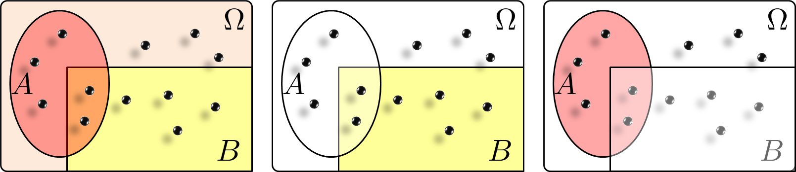
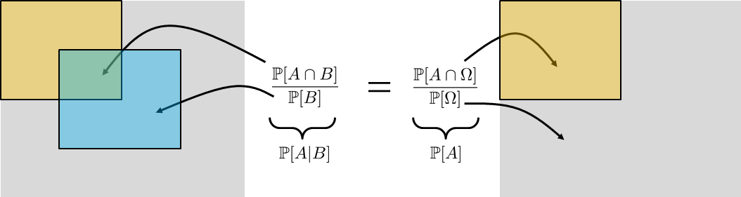
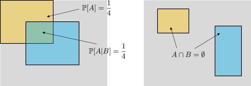
A pictorial illustration of independence is given in Figure 2.29. The key message is that if two events $A$ and $B$ are independent, then $\Pb[A|B] = \Pb[A]$. The conditional probability $\Pb[A|B]$ is the ratio of $\Pb[A\cap B]$ over $\Pb[B]$, which is the intersection over $B$ (the blue set). The probability $\Pb[A]$ is the yellow set over the sample space $\Omega$.

Disjoint versus independent

\mbox{Disjoint} \nLeftrightarrow \mbox{Independent}.

The statement says that disjoint and independent are two completely different concepts.

If $A$ and $B$ are disjoint, then $A \cap B = \emptyset$. This only implies that $\Pb[A \cap B] = 0$. However, it says nothing about whether $\Pb[A \cap B]$ can be factorized into $\Pb[A] \, \Pb[B]$. If $A$ and $B$ are independent, then we have $\Pb[A \cap B] = \Pb[A] \, \Pb[B]$. But this does not imply that $\Pb[A \cap B] = 0$. The only condition under which Disjoint $\Leftrightarrow$ Independence is when $\Pb[A] = 0$ or $\Pb[B] = 0$. Figure 2.30 depicts the situation. When two sets are independent, the conditional probability (which is a ratio) remains unchanged compared to unconditioned probability. When two sets are disjoint, they simply do not overlap.

**Figure 2.30.** Independent means that the conditional probability, which is a ratio, is the same as the unconditioned probability. Disjoint means that the two sets do not overlap.

Practice Exercise 2.15

Throw a die twice. Are $A$ and $B$ independent, where $$A = \{\mbox{1st die is 3}\} \quad\mbox{and}\quad B = \{\mbox{2nd die is 4}\}.$$

Solution

We can show that

\begin{aligned} \Pb[A \cap B] = \Pb[(3,4)] = \tfrac{1}{36}, \quad\quad \Pb[A] = \tfrac{1}{6}, \quad \mbox{and} \quad \Pb[B] = \tfrac{1}{6}. \end{aligned}

So $\Pb[A \cap B] = \Pb[A]\Pb[B]$. Thus, $A$ and $B$ are independent.

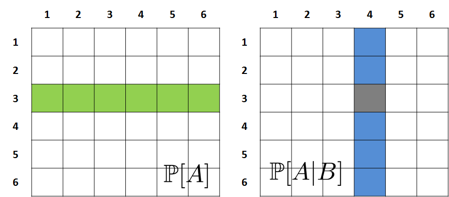
A pictorial illustration of this example is shown in Figure 2.31. The two events are independent because $A$ is one row in the 2D space, which yields a probability of $\frac{1}{6}$. The conditional probability $\Pb[A|B]$ is the coordinate $(3,4)$ over the event $B$, which is a column. It happens that $\Pb[A|B] = \frac{1}{6}$. Thus, the two events are independent.

Practice Exercise 2.16

Throw a die twice. Are $A$ and $B$ independent? $$A = \{\mbox{1st die is 3}\} \quad\mbox{and}\quad B = \{\mbox{sum is 7}\}.$$

Solution

Note that

\begin{aligned} \Pb[A \cap B] &= \Pb[(3,4)] = \tfrac{1}{36}, \qquad\qquad \Pb[A] = \tfrac{1}{6},\\ \Pb[B] &= \Pb[(1,6),(2,5),(3,4),(4,3),(5,2),(6,1)] = \tfrac{1}{6}. \end{aligned}

So $\Pb[A \cap B] = \Pb[A]\,\Pb[B]$. Thus, $A$ and $B$ are independent.

A pictorial illustration of this example is shown in Figure 2.32. Notice that whether the two events intersect is not how we determine independence (that only determines disjoint or not). The key is whether the conditional probability (which is the ratio) remains unchanged compared to the unconditioned probability.

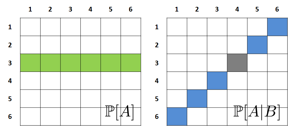
If we let $B = \{\mbox{sum is 8}\}$, then the situation is different. The intersection $A \cap B$ has a probability $\frac{1}{5}$ relative to $B$, and therefore $\Pb[A|B] = \frac{1}{5}$. Hence, the two events $A$ and $B$ are dependent. If you like a more intuitive argument, you can imagine that $B$ has happened, i.e., the sum is 8. Then the probability for the first die to be 1 is 0 because there is no way to construct 8 when the first die is 1. As a result, we have eliminated one choice for the first die, leaving only five options. Therefore, since $B$ has influenced the probability of $A$, they are dependent.

Practice Exercise 2.17

Throw a die twice. Let $$A = \{\mbox{max is 2}\} \quad\mbox{and}\quad B = \{\mbox{min is 2}\}.$$ Are $A$ and $B$ independent?

Solution

Let us first list out $A$ and $B$:

\begin{aligned} A &= \{(1,2), (2,1), (2,2)\},\\ B &= \{(2,2), (2,3), (2,4), (2,5), (2,6), (3,2), (4,2), (5,2), (6,2)\}. \end{aligned}

Therefore, the probabilities are

\begin{aligned} \Pb[A] &= \frac{3}{36}, \quad \Pb[B] = \frac{9}{36}, \quad\mbox{and}\quad \Pb[A \cap B] = \Pb[(2,2)] = \frac{1}{36}. \end{aligned}

Clearly, $\Pb[A \cap B] \not= \Pb[A]\Pb[B]$ and so $A$ and $B$ are dependent.

What is independence?

sep0ex
Two events are independent when the ratio $\Pb[A \cap B]/\Pb[B]$ remains unchanged compared to $\Pb[A]$.
Independence $\not=$ disjoint.

2.4.3Bayes' theorem and the law of total probability

Theorem 2.7 (Bayes' theorem)

For any two events $A$ and $B$ such that $\Pb[A] > 0$ and $\Pb[B] > 0$,

\Pb[A \,|\, B] = \frac{\Pb[B \,|\, A] \, \Pb[A]}{\Pb[B]}.

Proof. By the definition of conditional probabilities, we have

\begin{aligned} \Pb[A \,|\, B] = \frac{\Pb[A \cap B]}{\Pb[B]} \quad\mbox{and}\quad \Pb[B \,|\, A] = \frac{\Pb[B \cap A]}{\Pb[A]}. \end{aligned}

Rearranging the terms yields $$\Pb[A \,|\, B] \Pb[B] = \Pb[B \,|\, A]\Pb[A],$$ which gives the desired result by dividing both sides by $\Pb[B]$.

■

Bayes' theorem provides two views of the intersection $\Pb[A \cap B]$ using two different conditional probabilities. We call $\Pb[B \,|\, A]$ the conditional probability and $\Pb[A \,|\, B]$ the posterior probability. The order of $A$ and $B$ is arbitrary. We can also call $\Pb[A \,|\, B]$ the conditional probability and $\Pb[B \,|\, A]$ the posterior probability. The context of the problem will make this clear.

Bayes' theorem provides a way to switch $\Pb[A|B]$ and $\Pb[B|A]$. The next theorem helps us decompose an event into smaller events.

Theorem 2.8 (Law of Total Probability)

Let $\{A_1,\ldots,A_n\}$ be a partition of $\Omega$, i.e., $A_1,\ldots,A_n$ are disjoint and $\Omega = A_1 \cup \cdots \cup A_n$. Then, for any $B \subseteq \Omega$,

\Pb[B] = \sum_{i=1}^n \Pb[B \,|\, A_i] \; \Pb[A_i].

Proof. We start from the right-hand side.

\begin{aligned} \sum_{i=1}^n \Pb[B \,|\, A_i] \; \Pb[A_i] &\overset{(a)}{=} \sum_{i=1}^n \Pb[B \cap A_i] \overset{(b)}{=} \Pb\left[\bigcup_{i=1}^n (B \cap A_i)\right] \\ &\overset{(c)}{=} \Pb\left[B \cap \left(\bigcup_{i=1}^n A_i \right)\right] \overset{(d)}{=} \Pb[B \cap \Omega] = \Pb[B], \end{aligned}

where $(a)$ follows from the definition of conditional probability, $(b)$ is due to Axiom III, $(c)$ holds because of the distributive property of sets, and $(d)$ results from the partition property of $\{A_1,A_2,\ldots,A_n\}$.

■

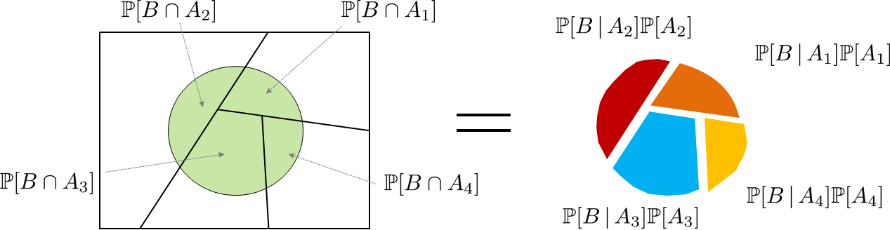
Interpretation. The law of total probability can be understood as follows. If the sample space $\Omega$ consists of disjoint subsets $A_1,\ldots,A_n$, we can compute the probability $\Pb[B]$ by summing over its portion $\Pb[B \cap A_1],\ldots,\Pb[B \cap A_n]$. However, each intersection can be written as

\Pb[B \cap A_i] = \Pb[B \,|\, A_i]\Pb[A_i].

In other words, we write $\Pb[B \cap A_i]$ as the conditional probability $\Pb[B \,|\, A_i]$ times the prior probability $\Pb[A_i]$. When we sum all of these intersections, we obtain the overall probability. See Figure 2.33 for a graphical portrayal.

**Figure 2.33.** The law of total probability decomposes the probability $\Pb[B]$ into multiple conditional probabilities $\Pb[B\,|\,A_i]$. The probability of obtaining each $\Pb[B\,|\,A_i]$ is $\Pb[A_i]$.

Corollary 2.4

Let $\{A_1,A_2,\ldots,A_n\}$ be a partition of $\Omega$, i.e., $A_1,\ldots,A_n$ are disjoint and $\Omega = A_1 \cup A_2 \cup \cdots \cup A_n$. Then, for any $B \subseteq \Omega$,

\Pb[A_j \,|\, B] = \frac{\Pb[B \, |\, A_j] \; \Pb[A_j]}{ \sum_{i=1}^n \Pb[B \,|\, A_i]\;\Pb[A_i]}.

Proof. The result follows directly from Bayes' theorem:

\begin{aligned} \Pb[A_j \,|\, B] &= \frac{\Pb[ B \,|\, A_j] \, \Pb[A_j]}{\Pb[B]} = \frac{\Pb[ B \,|\, A_j] \, \Pb[A_j]}{\sum_{i=1}^n \Pb[B \,|\, A_i] \; \Pb[A_i]}. \end{aligned}

■

Example 2.47

Suppose there are three types of players in a tennis tournament: $A$, $B$, and $C$. Fifty percent of the contestants in the tournament are $A$ players, 25% are $B$ players, and 25% are $C$ players. Your chance of beating the contestants depends on the class of the player, as follows:

\begin{aligned} & 0.3 \mbox{ against an $A$ player}\\ & 0.4 \mbox{ against a $B$ player}\\ & 0.5 \mbox{ against a $C$ player} \end{aligned}

If you play a match in this tournament, what is the probability of your winning the match? Supposing that you have won a match, what is the probability that you played against an $A$ player?

Solution

We first list all the known probabilities. We know from the percentage of players that

\begin{aligned} \Pb[A] = 0.5, \quad \Pb[B] = 0.25, \quad \Pb[C] = 0.25. \end{aligned}

Now, let $W$ be the event that you win the match. Then the conditional probabilities are defined as follows:

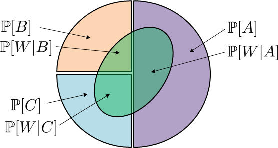
\begin{aligned} \Pb[W|A] = 0.3, \quad \Pb[W|B] = 0.4, \quad \Pb[W|C] = 0.5. \end{aligned}

Therefore, by the law of total probability, we can show that the probability of winning the match is

\begin{aligned} \Pb[W] &= \Pb[W \,|\, A]\,\Pb[A] + \Pb[W \,|\, B]\,\Pb[B] + \Pb[W \,|\, C]\,\Pb[C]\\ &= (0.3)(0.5) + (0.4)(0.25) + (0.5)(0.25) = 0.375. \end{aligned}

Given that you have won the match, the probability of $A$ given $W$ is

\begin{aligned} \Pb[A|W] &= \frac{\Pb[W|A]\Pb[A]}{\Pb[W]} = \frac{(0.3)(0.5)}{0.375} = 0.4. \end{aligned}

Example 2.48

Consider the communication channel shown below. The probability of sending a 1 is $p$ and the probability of sending a 0 is $1-p$. Given that 1 is sent, the probability of receiving 1 is $1-\eta$. Given that 0 is sent, the probability of receiving 0 is $1-\varepsilon$. Find the probability that a 1 has been correctly received.

Solution

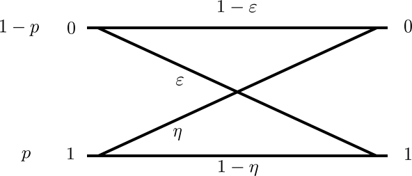
Define the events

\begin{aligned} S_0 &= \mbox{``0 is sent''}, \quad\mbox{and}\quad R_0 = \mbox{``0 is received''}.\\ S_1 &= \mbox{``1 is sent''}, \quad\mbox{and}\quad R_1 = \mbox{``1 is received''}. \end{aligned}

Then, the probability that 1 is received is $\Pb[R_1]$. However, $\Pb[R_1] \not= 1-\eta$ because $1-\eta$ is the conditional probability that 1 is received given that 1 is sent. It is possible that we receive 1 as a result of an error when 0 is sent. Therefore, we need to consider the probability that both $S_0$ and $S_1$ occur. Using the law of total probability we have

\begin{aligned} \Pb[R_1] &= \Pb[R_1 \,|\, S_1]\; \Pb[S_1] + \Pb[R_1 \,|\, S_0] \;\Pb[S_0]\\ &= (1-\eta)p + \varepsilon(1-p). \end{aligned}

Now, suppose that we have received 1. What is the probability that 1 was originally sent? This is asking for the posterior probability $\Pb[S_1 \,|\, R_1]$, which can be found using Bayes' theorem

\begin{aligned} \Pb[S_1 \,|\, R_1] &= \frac{\Pb[R_1 \,|\, S_1 ] \; \Pb[S_1]}{\Pb[R_1]} = \frac{(1-\eta)p}{(1-\eta)p + \varepsilon(1-p)}. \end{aligned}

When do we need to use Bayes' theorem and the law of total probability?

sep0ex
Bayes' theorem switches the role of the conditioning, from $\Pb[A|B]$ to $\Pb[B|A]$.

Example: $$\Pb[\text{win the game} \;|\; \text{play with A}] \quad\text{and}\quad \Pb[\text{play with A} \;|\; \text{win the game}].$$
The law of total probability decomposes an event into smaller events.

Example: $$\Pb[\text{win}] = \Pb[\text{win} \;|\; A]\Pb[A] + \Pb[\text{win} \;|\; B]\Pb[B].$$

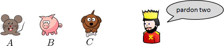
2.4.4The Three Prisoners problem

Now that you are familiar with the concepts of conditional probabilities, we would like to challenge you with the following problem, known as the Three Prisoners problem. If you understand how this problem can be resolved, you have mastered conditional probability.

Once upon a time, there were three prisoners $A$, $B$, and $C$. One day, the king decided to pardon two of them and sentence the last one, as in this figure:

**Figure 2.36.** The Three Prisoners problem: The king says that he will pardon two prisoners and sentence one.

One of the prisoners, prisoner $A$, heard the news and wanted to ask a friendly guard about his situation. The guard was honest. He was allowed to tell prisoner $A$ that prisoner $B$ would be pardoned or that prisoner $C$ would be pardoned, but he could not tell $A$ whether he would be pardoned. Prisoner $A$ thought about the problem, and he began to hesitate to ask the guard. Based on his present state of knowledge, his probability of being pardoned is $\tfrac{2}{3}$. However, if he asks the guard, this probability will be reduced to $\tfrac{1}{2}$ because the guard would tell him that one of the two other prisoners would be pardoned, and would tell him which one it would be. Prisoner A reasons that his chance of being pardoned would then drop because there are now only two prisoners left who may be pardoned, as illustrated in Figure 2.37:

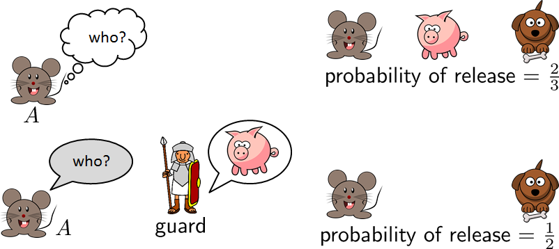
**Figure 2.37.** The Three Prisoners problem: If you do not ask the guard, your chance of being released is 2/3. If you ask the guard, the guard will tell you which one of the other prisoners will be released. Your chance of being released apparently drops to 1/2.

Should prisoner $A$ ask the guard? What has gone wrong with his reasoning? This problem is tricky in the sense that the verbal argument of prisoner $A$ seems flawless. If he asked the guard, indeed, the game would be reduced to two people. However, this does not seem correct, because regardless of what the guard says, the probability for $A$ to be pardoned should remain unchanged. Let's see how we can solve this puzzle.

Let $X_A$, $X_B$, $X_C$ be the events of sentencing prisoners $A$, $B$, $C$, respectively. Let $G_B$ be the event that the guard says that the prisoner $B$ is released. Without doing anything, we know that

\begin{aligned} \Pb[X_A] = \frac{1}{3}, \qquad \Pb[X_B] = \frac{1}{3}, \qquad \Pb[X_C] = \frac{1}{3}. \end{aligned}

Conditioned on these events, we can compute the following conditional probabilities that the guard says $B$ is pardoned:

\begin{aligned} \Pb[G_B \;|\; X_A ] = \frac{1}{2}, \qquad \Pb[G_B \;|\; X_B] = 0, \qquad \Pb[G_B \;|\; X_C ] = 1. \end{aligned}

Why are these conditional probabilities? $\Pb[G_B \;|\; X_B] = 0$ is quite straightforward. If the king decides to sentence $B$, the guard has no way of saying that $B$ will be pardoned. Therefore, $\Pb[G_B \;|\; X_B]$ must be zero. $\Pb[G_B \;|\; X_C] = 1$ is also not difficult. If the king decides to sentence $C$, then the guard has no choice but to tell you that $B$ will be pardoned, because the guard cannot say that $C$ will be pardoned and cannot say anything about prisoner $A$. Finally, $\Pb[G_B \;|\; X_A ] = \frac{1}{2}$ can be understood as follows: If the king decides to sentence $A$, the guard can either tell you $B$ or $C$. In other words, the guard flips a coin.

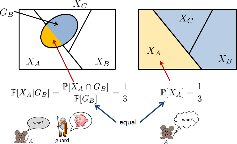
With these conditional probabilities ready, we can determine the probability. This is the conditional probability $\Pb[X_A \;|\; G_B]$. That is, supposing that the guard says $B$ is pardoned, what is the probability that $A$ will be sentenced? This is the actual scenario that $A$ is facing. Solving for this conditional probability is not difficult. By Bayes' theorem we know that

\begin{aligned} \Pb[X_A \;|\; G_B] = \frac{\Pb[G_B \;|\; X_A] \Pb[X_A]}{\Pb[G_B]}, \end{aligned}

and $\Pb[G_B] = \Pb[G_B|X_A]\Pb[X_A] + \Pb[G_B|X_B]\Pb[X_B] + \Pb[G_B|X_C]\Pb[X_C]$ according to the law of total probability. Substituting the numbers into these equations, we have that

\begin{aligned} \Pb[G_B] &= \Pb[G_B|X_A]\Pb[X_A] + \Pb[G_B|X_B]\Pb[X_B] + \Pb[G_B|X_C]\Pb[X_C]\\ &= \frac{1}{2} \times \frac{1}{3} + 0 \times \frac13 + 1 \times \frac13 = \frac{1}{2},\\ \Pb[X_A \;|\; G_B] &= \frac{\Pb[G_B \;|\; X_A] \Pb[X_A]}{\Pb[G_B]} = \frac{\frac{1}{2} \times \frac13 }{\frac{1}{2}} = \frac13. \end{aligned}

Therefore, given that the guard says $B$ is pardoned, the probability that $A$ will be sentenced remains $\frac13$. In fact, what you can show in this example is that $\Pb[X_A \;|\; G_B] = \frac13 = \Pb[X_A]$. Therefore, the presence or absence of the guard does not alter the probability. This is because what the guard says is independent of whether the prisoners will be pardoned. The lesson we learn from this problem is not to rely on verbal arguments. We need to write down the conditional probabilities and spell out the steps.

**Figure 2.38.** The Three Prisoners problem is resolved by noting that $\Pb[X_A|G_B] = \Pb[X_A]$. Therefore, the events $X_A$ and $G_B$ are independent.

How to resolve the Three Prisoners problem?

sep0ex
The key is that $G_A$, $G_B$, $G_C$ do not form a partition. See Figure 2.38.
$G_B \not= X_B$. When $G_B$ happens, the remaining set is not $X_A \cup X_C$.
The ratio $\Pb[X_A \cap G_B]/\Pb[G_B]$ equals $\Pb[X_A]$. This is independence.