eBook › Chapter 2 · Probability

Section 2.3

Axioms of Probability

We now turn to a deeper examination of the properties. Our motivation is simple. While the definition of probability law has achieved its goal of assigning a probability to an event, there must be restrictions on how the assignment can be made. For example, if we set $\Pb[\{H\}] = 1/3$, then $\Pb[\{T\}]$ must be $2/3$; otherwise, the sum of having a head and a tail will be greater than 1. The necessary restrictions on assigning a probability to an event are collectively known as the axioms of probability.

Definition 2.21 (Probability Law)

A probability law is a function $\Pb: \calF \rightarrow [0,1]$ that maps an event $A$ to a real number in $[0,\,1]$. The function must satisfy the axioms of probability:

I. Non-negativity: $\Pb[A] \ge 0$, for any $A \subseteq \Omega$.
II. Normalization: $\Pb[\Omega] = 1$.
III.
Additivity: For any disjoint sets $\{A_1,A_2,\ldots\}$, it must be true that
$\Pb\left[\bigcup_{i=1}^{\infty} A_i\right] = \sum_{i=1}^{\infty} \Pb[A_i].$

An axiom is a proposition that serves as a premise or starting point in a logical system. Axioms are not definitions, nor are they theorems. They are believed to be true or true within a certain context. In our case, the three axioms given above are those of Kolmogorov's probability. The Bayesian (or subjective) approach to probability relies on another set of axioms. We will not dive into the details of these historical issues; in this book, we will confine our discussion to the three axioms given above.

2.3.1Why these three probability axioms?

Why do we need three axioms? Why not just two axioms? Why these three particular axioms? The reasons are summarized in the box below.

Why these three axioms?

sep0ex
Axiom I (Non-negativity) ensures that probability is never negative.
Axiom II (Normalization) ensures that probability is never greater than 1.
Axiom III (Additivity) allows us to add probabilities when two events do not overlap.

Axiom I is called the non-negativity axiom. It ensures that a probability value cannot be negative. Non-negativity is a must for probability. It is meaningless to say that the probability of getting an event is a negative number.

Axiom II is called the normalization axiom. It ensures that the probability of observing all possible outcomes is 1. This gives the upper limit of the probability. The upper limit does not have to be 1. It could be 10 or 100. As long as we are consistent about this upper limit, we are good. However, for historical reasons and convenience, we choose 1 to be the upper limit.

Axiom III is called the additivity axiom and is the most critical one among the three. The additivity axiom defines how set operations can be translated into probability operations. In a nutshell, it says that if we have a set of disjoint events, the probabilities can be added. From the measure perspective, Axiom III makes sense because if $\Pb$ measures the size of an event, then two disjoint events should have their probabilities added. If two disjoint events do not allow their probabilities to be added, then there is no way to measure a combined event. Similarly, if the probabilities can somehow be added even for overlapping events, there will be inconsistencies because there is no systematic way to handle the overlapping regions.

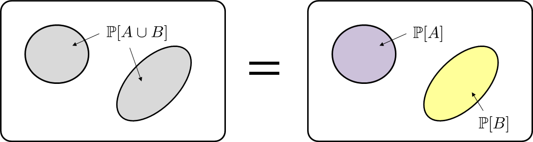
The countable additivity stated in Axiom III can be applied to both a finite number or an infinite number of sets. The finite case states that for any two disjoint sets $A$ and $B$, we have

\Pb[A \cup B] = \Pb[A] + \Pb[B].

In other words, if $A$ and $B$ are disjoint, then the probability of observing either $A$ or $B$ is the sum of the two individual probabilities. Figure 2.22 illustrates this idea.

Example 2.39

Let's see why Axiom III is critical. Consider throwing a fair die with $\Omega = \{\mydice{1}, \mydice{2},\mydice{3},\mydice{4},\mydice{5},\mydice{6}\}$. The probability of getting $\{\mydice{4},\mydice{6}\}$ is

\begin{aligned} \Pb[\{\mydice{4}, \mydice{6}\}] &= \Pb[\{\mydice{4}\} \cup \{\mydice{6}\}] = \Pb[\{\mydice{4}\}] + \Pb[\{\mydice{6}\}] = \frac{1}{6} + \frac{1}{6} = \frac{2}{6}. \end{aligned}

In this equation, the second equality holds because the events $\{\mydice{4}\}$ and $\{\mydice{6}\}$ are disjoint. If we do not have Axiom III, then we cannot add probabilities.

2.3.2Axioms through the lens of measure

Axioms are “rules” we must abide by when we construct a measure. Therefore, any valid measure must be compatible with the axioms, regardless of whether we have a weighting function or not. In the following two examples, we will see how the weighting functions are used in the axioms.

Example 2.40

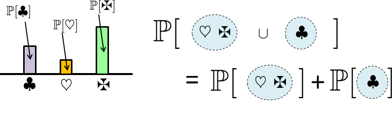
Consider a sample space with $\Omega = \{\clubsuit,\heartsuit,\maltese\}$. The probability for each outcome is

\begin{aligned} \Pb[\{\clubsuit\}] = \frac{2}{6}, \quad \Pb[\{\heartsuit\}] = \frac{1}{6}, \quad \Pb[\{\maltese\}] = \frac{3}{6}. \end{aligned}

Suppose we construct two disjoint events $E_1 = \{\clubsuit,\heartsuit\}$ and $E_2 = \{\maltese\}$. Then Axiom III says

\begin{aligned} \Pb[E_1 \cup E_2] &= \Pb[E_1] + \Pb[E_2] = \left(\frac{2}{6} + \frac{1}{6}\right) + \frac{3}{6} = 1. \end{aligned}

Note that in this calculation, the measure $\Pb$ is still a measure $\Pb$. If we endow it with a nonuniform weight function, then $\Pb$ applies the corresponding weights to the corresponding outcomes. This process is compatible with the axioms. See Figure 2.23 for a pictorial illustration.

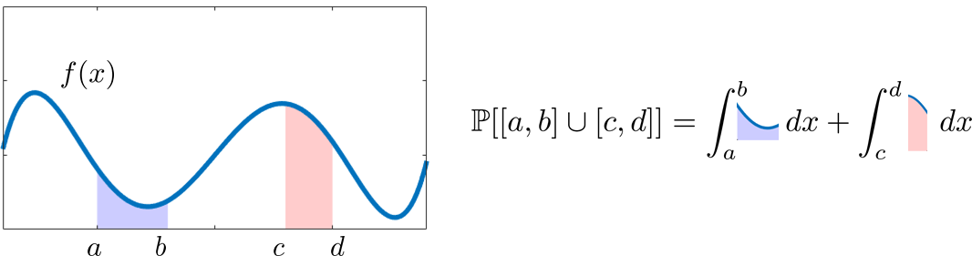
**Figure 2.23.** Applying weighting functions to the measures: Suppose we have three elements in the set. To compute the probability $\Pb[\{\heartsuit,\maltese\} \cup \{\clubsuit\}]$, we can write it as the sum of $\Pb[\{\heartsuit,\maltese\}]$ and $\Pb[\{\clubsuit\}]$.

Example 2.41

Suppose the sample space is an interval $\Omega = [0,1]$. The two events are $E_1 = [a,b]$ and $E_2 = [c,d]$. Assume that the measure $\Pb$ uses a weighting function $f(x)$. Then, by Axiom III, we know that

\begin{aligned} \Pb[E_1 \cup E_2] &= \Pb[E_1] + \Pb[E_2] \\ &= \Pb[[a,b]] + \Pb[[c,d]] \qquad\qquad\quad \text{(by Axiom 3)}\\ &= \int_a^b f(x)\;dx + \int_c^d f(x) \;dx, \qquad \text{(apply the measure)}. \end{aligned}

As you can see, there is no conflict between the axioms and the measure. Figure 2.24 illustrates this example.

2.3.3Corollaries derived from the axioms

The union of $A$ and $B$ is equivalent to the logical operator “OR”. Once the logical operation “OR” is defined, all other logical operations can be defined. See the following examples.

Corollary 2.1

Let $A \in \calF$ be an event. Then,

(a) $\Pb[A^c] = 1 - \Pb[A]$.
(b) $\Pb[A] \le 1$.
(c) $\Pb[\emptyset] = 0$.

Proof. (a) Since $\Omega = A \cup A^c$, by finite additivity we have $\Pb[\Omega] = \Pb[A \cup A^c] = \Pb[A] + \Pb[A^c]$. By the normalization axiom, we have $\Pb[\Omega] = 1$. Therefore, $\Pb[A^c] = 1 - \Pb[A]$.

(b) We prove by contradiction. Assume $\Pb[A] > 1$. Consider the complement $A^c$ where $A \cup A^c = \Omega$. Since $\Pb[A^c] = 1-\Pb[A]$, we must have $\Pb[A^c] < 0$ because by hypothesis $\Pb[A] > 1$. But $\Pb[A^c] < 0$ violates the non-negativity axiom. So we must have $\Pb[A] \le 1$.

■

Corollary 2.2 (Unions of Two Non-Disjoint Sets)

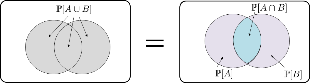
For any $A$ and $B$ in $\calF$,

\Pb[A \cup B] = \Pb[A] + \Pb[B] - \Pb[A \cap B].

This statement is different from Axiom III because $A$ and $B$ are not necessarily disjoint.

Proof. First, observe that $A \cup B$ can be partitioned into three disjoint subsets as $A \cup B = (A \backslash B) \cup (A \cap B) \cup (B \backslash A)$. Since $A \backslash B = A \cap B^c$ and $B \backslash A = B \cap A^c$, by finite additivity we have that

\begin{aligned} \Pb[A \cup B] &= \Pb[A \backslash B] + \Pb[A \cap B] + \Pb[B \backslash A] = \Pb[A \cap B^c] + \Pb[A \cap B] + \Pb[B \cap A^c] \\ &\overset{(a)}{=} \Pb[A \cap B^c] + \Pb[A \cap B] + \Pb[B \cap A^c] + \Pb[A \cap B] - \Pb[A \cap B]\\ &\overset{(b)}{=} \Pb[A \cap (B^c \cup B)] + \Pb[(A^c \cup A) \cap B] - \Pb[A \cap B]\\ &= \Pb[A \cap \Omega] + \Pb[\Omega \cap B] - \Pb[A \cap B] = \Pb[A] + \Pb[B] - \Pb[A \cap B], \end{aligned}

where in (a) we added and subtracted a term $\Pb[A \cap B]$, and in (b) we used finite additivity so that $\Pb[A \cap B^c] + \Pb[A \cap B] = \Pb[(A \cap B^c) \cup (A \cap B)] = \Pb[A \cap (B^c \cup B)]$.

■

**Figure 2.25.** For any $A$ and $B$, $\Pb[A \cup B] = \Pb[A] + \Pb[B] - \Pb[A \cap B]$.

Example 2.42

The corollary is easy to understand if we consider the following example. Let $\Omega = \{\mydice{1}, \mydice{2},\mydice{3},\mydice{4},\mydice{5},\mydice{6}\}$ be the sample space of a fair die. Let $A = \{\mydice{1}, \mydice{2},\mydice{3}\}$ and $B = \{\mydice{3},\mydice{4},\mydice{5}\}$. Then

\begin{aligned} \Pb[A \cup B] &= \Pb[\{\mydice{1}, \mydice{2},\mydice{3},\mydice{4},\mydice{5}\}] = \frac{5}{6}. \end{aligned}

We can also use the corollary to obtain the same result:

\begin{aligned} \Pb[A \cup B] &= \Pb[A] + \Pb[B] - \Pb[A\cap B] \\ &= \Pb[\{\mydice{1}, \mydice{2},\mydice{3}\}] + \Pb[\{\mydice{3},\mydice{4},\mydice{5}\}] - \Pb[\{\mydice{3}\}]\\ &= \frac{3}{6} + \frac{3}{6} - \frac{1}{6} = \frac{5}{6}. \end{aligned}

Corollary 2.3 (Inequalities)

Let $A$ and $B$ be two events in $\calF$. Then,

(a) $\Pb[A \cup B] \le \Pb[A] + \Pb[B]$. (Union Bound)
(b) If $A \subseteq B$, then $\Pb[A] \le \Pb[B]$.

Proof. (a) Since $\Pb[A \cup B] = \Pb[A] + \Pb[B] - \Pb[A \cap B]$ and by non-negativity axiom $\Pb[A \cap B] \ge 0$, we must have $\Pb[A \cup B] \le \Pb[A] + \Pb[B]$. (b) If $A \subseteq B$, then there exists a set $B \backslash A$ such that $B = A \cup (B \backslash A)$. Therefore, by finite additivity we have $\Pb[B] = \Pb[A] + \Pb[B \backslash A] \ge \Pb[A]$. Since $\Pb[B \backslash A] \ge 0$, it follows that $\Pb[A] + \Pb[B \backslash A] \ge \Pb[A]$. Thus we have $\Pb[B] \ge \Pb[A]$.

■

Union bound is a frequently used tool for analyzing probabilities when the intersection $A \cap B$ is difficult to evaluate. Part (b) is useful when considering two events of different “sizes.” For example, in the bus-waiting example, if we let $A = \{t \le 5\}$, and $B = \{t \le 10\}$, then $\Pb[A] \le \Pb[B]$ because we have to wait for the first 5 minutes to go into the remaining 5 minutes.

Practice Exercise 2.13

Let the events $A$ and $B$ have $\Pb[A] = x$, $\Pb[B] = y$ and $\Pb[A\cup B] = z$. Find the following probabilities: $\Pb[A\cap B]$, $\Pb[A^c \cup B^c]$, and $\Pb[A\cap B^c]$.

Solution

(a) Note that $z = \Pb[A\cup B]=\Pb[A]+\Pb[B]-\Pb[A\cap B]$. Thus, $\Pb[A \cap B] = x+y-z.$
(b)
We can take the complement to obtain the result:
$\begin{aligned} \Pb[A^c\cup B^c] &= 1-\Pb[(A^c\cup B^c)^c] =1-\Pb[A \cap B]=1-x-y+z. \end{aligned}$
(c) $\Pb[A \cap B^c]=\Pb[A]-\Pb[A\cap B]=x-(x+y-z)=z-y$.

Practice Exercise 2.14

Consider a sample space $$\Omega = \{f: \R \rightarrow \R \,|\, f(x) = ax, \text{for all } a \in \R, x \in \R\}.$$ There are two events: $A = \{f \,|\, f(x) = ax, \; a \ge 0\}$, and $B = \{f \,|\, f(x) = ax, \; a \le 0\}$. So, basically, $A$ is the set of all straight lines with positive slope, and $B$ is the set of straight lines with negative slope. Show that the union bound is tight.

Solution

First of all, we note that $$\Pb[A \cup B] = \Pb[A] + \Pb[B] - \Pb[A \cap B].$$ The intersection is $$\Pb[A \cap B] = \Pb[\{f \,|\, f(x) = 0\}].$$ Since this is a point set in the real line, it has measure zero. Thus, $\Pb[A \cap B] = 0$ and hence $\Pb[A \cup B] = \Pb[A] + \Pb[B]$. So the union bound is tight.

Closing remark. The development of today's probability theory is generally credited to Andrey Kolmogorov's 1933 book Foundations of the Theory of Probability. We close this section by citing one of the tables of the book. The table summarizes the correspondence between set theory and random events.

Theory of sets	Random events
lightgray $A$ and $B$ are disjoint, i.e., $A \cap B = \emptyset$	Events $A$ and $B$ are incompatible
$A_1 \cap A_2 \cdots \cap A_N = \emptyset$	Events $A_1,\ldots,A_N$ are incompatible
lightgray $A_1 \cap A_2 \cdots \cap A_N = X$	Event $X$ is defined as the simultaneous occurrence of events $A_1,\ldots,A_N$
$A_1 \cup A_2 \cdots \cup A_N = X$	Event $X$ is defined as the occurrence of at least one of the events $A_1,\ldots,A_N$
lightgray $A^c$	The opposite event $A^c$ consisting of the non-occurrence of event $A$
$A = \emptyset$	Event $A$ is impossible
lightgray $A = \Omega$	Event $A$ must occur
$A_1,\ldots,A_N$ form a partition of $\Omega$	The experiment consists of determining which of the events $A_1,\ldots,A_N$ occurs
lightgray $B \subset A$	From the occurrence of event $B$ follows the inevitable occurrence of $A$

Table 2.2. Kolmogorov's summary of set theory results and random events.

Theory of sets	Random events
lightgray \(A\) and \(B\) are disjoint, i.e., \(A \cap B = \emptyset\)	Events \(A\) and \(B\) are incompatible
\(A_1 \cap A_2 \cdots \cap A_N = \emptyset\)	Events \(A_1,\ldots,A_N\) are incompatible
lightgray \(A_1 \cap A_2 \cdots \cap A_N = X\)	Event \(X\) is defined as the simultaneous occurrence of events \(A_1,\ldots,A_N\)
\(A_1 \cup A_2 \cdots \cup A_N = X\)	Event \(X\) is defined as the occurrence of at least one of the events \(A_1,\ldots,A_N\)
lightgray \(A^c\)	The opposite event \(A^c\) consisting of the non-occurrence of event \(A\)
\(A = \emptyset\)	Event \(A\) is impossible
lightgray \(A = \Omega\)	Event \(A\) must occur
\(A_1,\ldots,A_N\) form a partition of \(\Omega\)	The experiment consists of determining which of the events \(A_1,\ldots,A_N\) occurs
lightgray \(B \subset A\)	From the occurrence of event \(B\) follows the inevitable occurrence of \(A\)