eBook › Chapter 9 · Confidence and Hypothesis

Section 9.4

Neyman-Pearson Test

The hypothesis testing procedures we discussed in the previous section are elementary in the sense that we have not discussed much theory. This section aims to fill the gap so that you can understand hypothesis testing from a broader perspective. This generalization will also help to bridge statistics to other disciplines such as classification in machine learning and detection in signal processing. We call this theoretical analysis the Neyman-Pearson framework.

9.4.1Null and alternative distributions

When we discussed hypothesis testing in the previous section, we focused exclusively on the null hypothesis $H_0$. Regardless of whether we are studying the $Z$-test or the $T$-test, using the critical value or the $p$-value, all the distributions are associated with the distribution under $H_0$.

What do we mean by “distribution under $H_0$”? Using $\widehat{\Theta}$ as an example, the PDF of $\widehat{\Theta}$ is assumed to be $\text{Gaussian}(\theta,\sigma^2/N)$. This Gaussian, centered at $\theta$, is the distribution assumed under $H_0$. As we decide whether to keep or reject $H_0$, we look at the critical value and the $p$-value of the test statistic under $\text{Gaussian}(\theta,\sigma^2/N)$.

Importantly, the analysis of hypothesis testing is not just about $H_0$ — it is also about the alternative hypothesis $H_1$, which uses a different PDF. For example, $H_1$ could use $\text{Gaussian}(\theta',\sigma^2/N)$ for $\theta' > \theta$. Therefore, for the same testing statistic $\Thetahat$, we can check how close it is to $H_1$.

To capture both distributions, we define

\begin{aligned} f_0(y) &= f_Y(y \; |\; H_0),\\ f_1(y) &= f_Y(y \; |\; H_1). \end{aligned}

The first PDF defines the distribution when the true model is $H_0$. The second PDF is the distribution when the true model is $H_1$.

Example 9.11

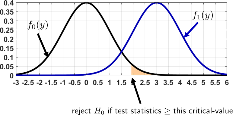
Consider an estimator $Y \sim \text{Gaussian}(\theta, \sigma^2/N)$. Define two hypotheses $H_0: \theta = 120$ and $H_1: \theta > 120$. The two PDFs are then

\begin{aligned} f_0(y) &= f_{Y}(y | H_0) = \text{Gaussian}(120, \sigma^2/N), \\ f_1(y) &= f_{Y}(y | H_1) = \text{Gaussian}(\theta', \sigma^2/N), \quad \theta'>120. \end{aligned}

A graph of the two distributions is shown in Figure 9.17. In this figure we plot the PDF under the null hypothesis and the PDF under an alternative hypothesis. The decision is based on the null, where we marked the critical value.

Students are frequently confused about the exact equation of the PDF under $H_1$. If the alternative hypothesis is defined as $\theta > 120$, shall we define the PDF as a Gaussian centered at 130 or 151.4? They are both valid alternative hypotheses. The answer is that we are going to express all equations based on $\theta'$. For example, if we want to analyze the prediction error (this term will be explained later), the prediction error will be a function of $\theta'$. If $\theta'$ is close to $\theta$, we will expect a larger prediction error. However, if $\theta'$ is far away from $\theta$, the prediction error may be small.

Whenever we discuss hypothesis testing, a decision rule is always implied. A decision rule is a mapping $\delta(\cdot)$ from sample space $\calY$ of the test statistic $Y$ (or $\Thetahat$ if you prefer) to the binary space of $\{0, 1\}$:

\delta(y) = \begin{cases} 1, &\qquad\text{if}\quad y \in R_\alpha, \quad (\text{we will reject $H_0$}),\\ 0, &\qquad\text{if}\quad y \not\in R_\alpha, \quad (\text{we will keep $H_0$}). \end{cases}

Here $R_\alpha$ is the rejection zone. For example, in a one-sided testing at a critical level $\alpha$, the rejection zone is $R_\alpha = \{y \ge \Phi^{-1}(1-\alpha)\}$. Therefore, as long as $y \ge \Phi^{-1}(1-\alpha)$, we will reject the null hypothesis. Otherwise, we will keep the null hypothesis. A rejection zone can be one-sided, two-sided, or even more complicated.

Example 9.12

Consider $H_0: \theta = 0.35$ and $H_1: \theta > 0.35$. It was found that the sample average over $1009$ samples is $\Thetahat = 0.387$, with $\sigma^2 = 0.227$. The normalized test statistic is $\widehat{Z} = \sqrt{N}(\Thetahat - \theta)/\sigma = 2.432$. At a 5% critical level, define the decision rule based on the critical-value approach.

Solution

If $\alpha = 0.05$, it follows that $z_\alpha = \Phi^{-1}(1-0.05) = 1.65$. Therefore, the decision rule is

\delta(\widehat{z}) = \begin{cases} 1, &\qquad\text{if}\quad \widehat{z} \ge 1.65, \quad (\text{we will reject $H_0$}),\\ 0, &\qquad\text{if}\quad \widehat{z} < 1.65, \quad (\text{we will keep $H_0$}), \end{cases}

where $\widehat{z}$ is the realization of $\widehat{Z}$. In this particular problem, we have $\widehat{z} = 2.432$. Thus, according to the decision rule, we need to reject $H_0$.

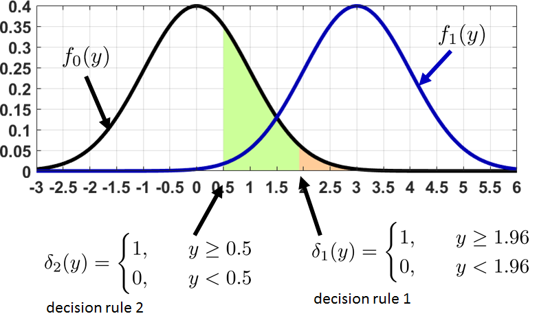
A decision rule is something you create. You do not need to follow the critical-value or the $p$-value procedure — you can create your own decision rule. For example, you can say “reject $H_0$ when $|y| > 0.000001$”. There is nothing wrong with this decision rule except that you will almost always reject the null hypothesis (so it is a bad decision rule). See Figure 9.18 for a graph of a similar example. If you follow the critical-value or the $p$-value procedures, it turns out that the resulting decision rule is equivalent to some form of optimal decision rule. This concept is the Neyman-Pearson framework, which we will explain shortly.

**Figure 9.18.** Two possible decision rules $\delta_1(y)$ and $\delta_2(y)$. In this example, $\delta_1(y)$ is designed according to the critical-value approach at $\alpha = 0.025$, whereas $\delta_2(y)$ is arbitrarily designed. Both are valid decision rules, although $\delta_2$ should not be used because it tends to reject the null hypothesis more often than desired.

9.4.2Type 1 and type 2 errors

Since hypothesis testing is about applying a decision rule to the test statistics, and since no decision rule is perfect, it is natural to ask about the error expected from a particular decision rule. In this subsection we define the decision error. However, the terminology varies from discipline to discipline. We will explain the decision error first through the statistics perspective and then through the signal processing perspective.

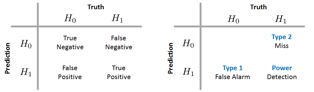
Two tables of the cases that can be generated by a binary decision-making process are shown in Figure 9.19. The columns of the tables are the true statements, i.e., whether the test statistic has a population distribution under $H_0$ or $H_1$. The rows of the tables are the statements predicted by the decision rule, i.e., whether we should declare the statistics are from $H_0$ or $H_1$. Each combination of the truth and prediction has a label:

sep0ex
True positive: The truth is $H_1$, and you declare $H_1$.
True negative: The truth is $H_0$, and you declare $H_0$.
False positive: The truth is $H_0$, and you declare $H_1$.
False negative: The truth is $H_1$, and you declare $H_0$.

Different communities have different ways of labeling these quantities. In the statistics community the false negative rate (i.e., the number of false negative cases divided by the total number of cases) is called the type 2 error, and the false positive rate is called the type 1 error. The true positive rate is called the power of the decision rule.

In the engineering community (e.g., radar engineering and signal processing) the objective is to detect whether a target (e.g., a missile or an enemy aircraft) is present. In this context, the false positive rate is known as the probability of false alarm, since personnel will be alerted when no target is present. The false negative rate is known as the probability of miss because you miss a target. If the truth is $H_1$ and the prediction is also $H_1$, we call this the probability of detection.

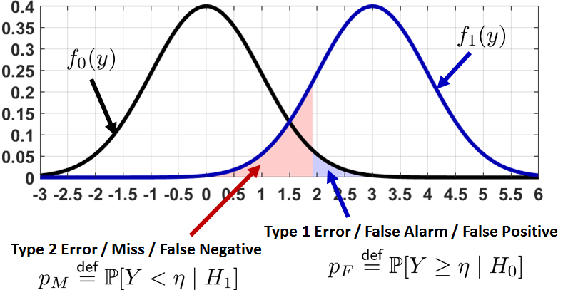
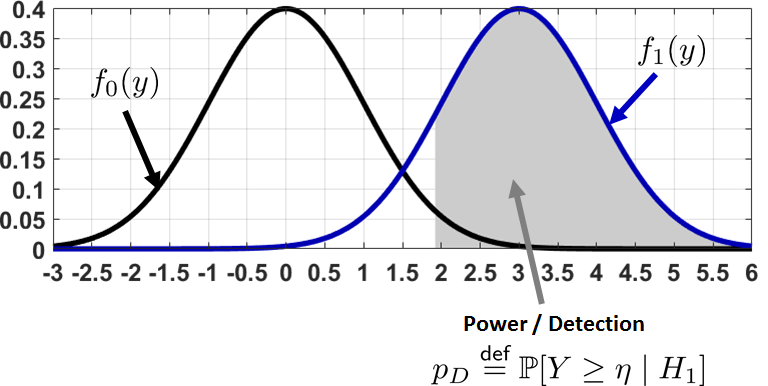
**Figure 9.19.** Terminology used in labeling the prediction error. The terms “Type 1 error” and “Type 2 error” are commonly used by the statistics community, whereas the terms “false alarm”, “miss” and “detection” are more often used in the engineering community.

The diagram in Figure 9.20 will help to clarify these definitions. Given two hypotheses $H_0$ and $H_1$, there exist the corresponding distributions $f_0(y)$ and $f_1(y)$, which are the PDFs of the test statistics $Y$ (or $\Thetahat$ if you prefer). Supposing that our decision rule is to declare $H_1$ when $Y \ge \eta$ for some $\eta$, for example, $\eta = 1.65$ for a 5% critical level, there are two areas under the curve that we need to consider.

sep0ex
Type 1 / False alarm. The blue region under the curve represents the probability of declaring $H_1$ (i.e., we choose to reject the null) while the truth is actually $H_0$ (i.e., we should not have rejected the null). Mathematically, this probability is
$\begin{aligned} p_F &= \Pb[Y \ge \eta \;|\; H_0] = \int_{y \ge \eta} f_0(y)\;dy. \end{aligned}$
Type 2 / Miss. The pink region under the curve represents the probability of declaring $H_0$ (i.e., we choose to keep the null) while the truth is actually $H_1$ (i.e., we should have rejected the null). Mathematically, this probability is
$\begin{aligned} p_M &= \Pb[Y < \eta \;|\; H_1] = \int_{y < \eta} f_1(y)\;dy. \end{aligned}$

The power of the decision rule is also known as the detection. It is defined as

p_D = \Pb[Y \ge \eta \;|\; H_1].

A plot illustrating the power of the decision rule is shown in Figure 9.21. Since $p_D$ is the conditional probability of $Y \ge \eta$ given $H_1$, it is the complement of $p_M$, and so we have the identity

$$p_D = 1-p_M.$$

Some communities refer to the above quantities in terms of the counts instead of the probabilities. The difference is that the probabilities are normalized to $[0,1]$ whereas the counts are just the raw integers obtained from running an experiment. We prefer to use the probabilities because they are the theoretical values. If you tell us the distributions $f_0$ and $f_1$, we can report the probabilities. The counts, by contrast, are just another form of sample statistics. The number of counts today may be different from the number of counts tomorrow because they are obtained from the experiments. The difference between probabilities and counts is analogous to the difference between PMFs and histograms.

Since the probability of errors changes as the decision rule changes, it is necessary to define $p_F$, $p_D$ and $p_M$ as functions of $\delta$. In addition, hypothesis testing is not limited to one-sided tests. We can define the rejection zone as $R_\alpha = \{y \;|\; \text{reject$H_0$using a critical level$$}\}$. The probabilities $p_F$ and $p_M$ are defined as

\begin{aligned} p_F(\delta) &= \int \delta(y) f_0(y)\;dy = \int_{y \in R_\alpha} f_0(y)\;dy,\\ p_M(\delta) &= \int (1-\delta(y)) f_1(y)\;dy = \int_{y \not\in R_\alpha} f_1(y)\;dy. \end{aligned}

Using the property that $p_D = 1-p_M$, we have that

p_D(\delta) = 1-p_M(\delta) = \int_{y \in R_\alpha} f_1(y)\;dy.

Note that the rejection zone does not need to depend on $\alpha$. You can arbitrarily define the rejection zone, and the probabilities $p_F$, $p_M$, and $p_D$ can still be defined.

Example 9.13

Find $p_F(\delta_1)$ and $p_F(\delta_2)$ for the decision rule in Figure 9.18.

Solution

Since $f_0$ is a Gaussian with zero mean and unit variance, it follows that

\begin{aligned} p_F(\delta_1) &= \int_{1.96}^{\infty} \frac{1}{\sqrt{2\pi}}e^{-\frac{y^2}{2}} \;dy = 1-\Phi(1.96) = 0.025,\\ p_F(\delta_2) &= \int_{0.5}^{\infty} \frac{1}{\sqrt{2\pi}}e^{-\frac{y^2}{2}} \;dy = 1-\Phi(0.5) = 0.3085. \end{aligned}

9.4.3Neyman-Pearson decision

At this point you have probably observed something about the critical-value test and the $p$-value test. Among the four types of decision combinations, we are looking at the false positive rate, or the probability of false alarm $p_F(\delta)$. The critical-value test requires us to find $\delta$ such that $p_F(\delta)$ is equal to $\alpha$. That is, if you tell us the critical level $\alpha$ (e.g., $\alpha = 0.05$), we will find a decision rule (by telling you the cutoff) such that the false alarm rate is $\alpha$. Consider an example:

Example 9.14

Let $\alpha = 0.05$. Assume that $f_0$ is a Gaussian with zero-mean and unit-variance. Let us do a one-sided test for $H_0: \theta = 0$ versus $H_1: \theta > 0$. Find $\delta$ such that $p_F(\delta) = \alpha$.

Solution

Let the decision rule $\delta$ be

\begin{aligned} \delta(y) = \begin{cases} 1, &\; y \ge \eta,\\ 0, &\; y < \eta. \end{cases} \end{aligned}

Our goal is to find $\eta$. The probability of false alarm is

\begin{aligned} p_F(\delta) = \int_{\eta}^{\infty} \frac{1}{\sqrt{2\pi}} e^{ -\frac{y^2}{2} } \;dy = 1-\Phi(\eta). \end{aligned}

Equating this to $\alpha$, it follows that $1-\Phi(\eta) = \alpha$ implies $\eta = \Phi^{-1}(1-\alpha) = 1.65$. So the decision rule becomes

\delta(y) = \begin{cases} 1, &\qquad y \ge 1.65,\\ 0, &\qquad y < 1.65. \end{cases}

If you apply this decision rule, you are guaranteed that the false alarm rate is $\alpha = 0.05$.

But why should we aim for $p_F(\delta)$ equal to $\alpha$? Isn't a lower false alarm rate better? Indeed, we would not mind having a lower false alarm, so we are happy to have any $\delta$ that satisfies $p_F(\delta) \le \alpha$. However, changing the equality to an inequality means that we now have a set of $\delta$ instead of a unique $\delta$. More importantly, we need to pay attention to the trade-off between $p_F(\delta)$ and $p_D(\delta)$. The smaller the $p_F(\delta)$ a decision rule $\delta$ provides, the smaller the $p_D(\delta)$ you can achieve. This is immediately apparent from Figure 9.20 and Figure 9.21. (If you move the cutoff to the right, the gray area and the blue area will both shrink.) Therefore, the desired optimization should be formulated as: From all the decision rules $\delta$ that have a false alarm rate of no larger than $\alpha$, we pick the one that maximizes the detection rate. The resulting decision rule is known as the Neyman-Pearson decision rule.

Definition 9.2

The Neyman-Pearson decision rule is defined as the solution to the optimization

\begin{aligned} \delta^* &= \argmax{\delta}\;\; p_D(\delta), \\ &\quad \text{subject to} \;\; p_F(\delta)\le \alpha. \end{aligned}

Figure 9.22 illustrates two decision rules $\delta^*(y)$ and $\delta(y)$. The first decision rule $\delta^*(y)$ is obtained according to the critical-value approach, with $\alpha = 0.025$. As we will prove shortly, this is also the optimal Neyman-Pearson decision rule for a one-sided hypothesis test at $\alpha = 0.025$. The second decision rule $\delta(y)$ has a harsher cutoff, meaning that you need an extreme test statistic to reject the null hypothesis. Clearly, the $p$-value obtained by $\delta(y)$ is less than $\alpha = 0.025$. Thus, $\delta(y)$ is a valid decision rule according to the Neyman-Pearson formulation. However, $\delta(y)$ is not optimal because the detection rate is not maximized.

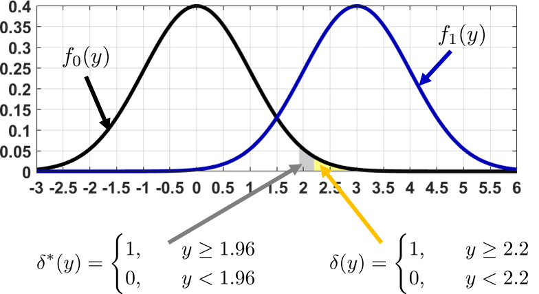
Because of the complementary behavior of $p_F$ and $p_D$, it follows that $p_D$ is maximized when $p_F$ hits the upper bound. If we want to maximize the detection rate we need to stretch the false alarm rate as much as possible. As a result, the Neyman-Pearson solution occurs when $p_F(\delta) = \alpha$, i.e., when the equality is met.

The Neyman-Pearson framework is a general framework for all distributions $f_0$ and $f_1$, as opposed to the critical-value and $p$-value examples, which are either Gaussian or Student's $t$-distribution. The solution to the Neyman-Pearson optimization is a decision rule known as the likelihood ratio test. The likelihood ratio is defined as follows.

Definition 9.3

The likelihood ratio for two distributions $f_1(y)$ and $f_0(y)$ is

L(y) = \frac{f_1(y)}{f_0(y)}.

It turns out that the solution to the Neyman-Pearson optimization takes the form of the likelihood ratio.

Theorem 9.2

The solution to the Neyman-Pearson optimization is a decision rule that checks the likelihood ratio

\begin{aligned} \delta^*(y) = \begin{cases} 1, &\qquad L(y) \ge \eta,\\ 0, &\qquad L(y) < \eta, \end{cases} \end{aligned}

for some decision boundary $\eta$ which is a function of the critical level $\alpha$.

What is so special about Neyman-Pearson decision rule?

sep0ex
It is the optimal decision. Its optimality is defined w.r.t. maximizing the detection rate while keeping a reasonable false alarm rate:
$\begin{aligned} \delta^* &= \argmax{\delta}\;\; p_D(\delta), \\ &\quad \text{subject to} \;\; p_F(\delta)\le \alpha. \end{aligned}$
If your goal is to maximize the detection rate while maintaining the false alarm rate, you cannot do better than Neyman-Pearson.
Its solution is the likelihood ratio test:
$\delta^*(y) = \begin{cases} 1, &\qquad L(y) \ge \eta,\\ 0, &\qquad L(y) < \eta, \end{cases}$
where $L(y) = f_1(y)/f_0(y)$ is the likelihood ratio.
The critical-value test and the $p$-value test are special cases of the Neyman-Pearson test.

Deriving the solution to the Neyman-Pearson optimization can be skipped if this is your first time reading the book.

Proof. Given $\alpha$, choose $\delta^*$ such that the false alarm rate is maximized: $p_F(\delta^*) = \alpha$. Then, by substituting the definition of $\delta^*$ into the false alarm rate,

\begin{aligned} \alpha = p_F(\delta^*) &= \int_{-\infty}^{\infty} \delta^*(y) f_0(y) \;dy \\ &= \int_{L(y) \ge \eta} 1 \cdot f_0(y) \;dy + \int_{L(y) < \eta} 0 \cdot f_0(y) \;dy. \end{aligned}

Now, consider another decision rule $\delta$ that is not optimal but is feasible. That means that $\delta$ satisfies $p_F(\delta) \le \alpha$. Therefore,

\begin{aligned} \alpha \ge p_F(\delta) &= \int_{-\infty}^{\infty} \delta(y) f_0(y) \;dy \\ &= \int_{L(y) \ge \eta} \delta(y) \cdot f_0(y) \;dy + \int_{L(y) < \eta} \delta(y) \cdot f_0(y) \;dy. \end{aligned}

Our goal is to show that $p_D(\delta^*) \ge p_D(\delta)$, because by proving this result we can claim that $\delta^*$ maximizes the detection rate.

By combining Eq. (9.33) and Eq. (9.34), we have

\begin{aligned} 0 &\le p_F(\delta^*) - p_F(\delta) \\ &= \int_{L(y)\ge \eta} (1-\delta(y)) f_0(y) \;dy - \int_{L(y) < \eta} \delta(y) f_0(y) \;dy. \end{aligned}

Define $L(y) = \frac{f_1(y)}{f_0(y)}$. Then $L(y)\ge \eta$ if and only if $f_1(y) \ge \eta f_0(y)$. So,

\begin{aligned} p_D(\delta^*) - p_D(\delta) &= \int_{L(y)\ge \eta} (1-\delta(y))f_1(y) \;dy - \int_{L(y) < \eta} \delta(y)f_1(y) \;dy \\ &= \int_{L(y)\ge \eta} (1-\delta(y))\eta f_0(y) \;dy - \int_{L(y) < \eta} \delta(y) \eta f_0(y) \;dy \\ &= \eta \left[\int_{L(y)\ge \eta} (1-\delta(y))f_0(y) \;dy - \int_{L(y) < \eta} \delta(y)f_0(y) \;dy\right] \ge 0, \end{aligned}

where the last inequality holds because of Eq. (9.35). Therefore, we conclude that $\delta^*$ maximizes $p_D$.

■

End of the proof. Please join us again.

At this point, you may object that the likelihood ratio test (i.e., the Neyman-Pearson decision rule) is very different from the hypothesis testing examples we have seen in the previous section because now we need to handle the likelihood ratio $L(y)$. Rest assured that they are the same, as illustrated by the following example.

Example 9.15

Consider two hypotheses: $H_0: Y \sim \text{Gaussian}(0,\sigma^2)$, and $H_1: Y \sim \text{Gaussian}(\mu,\sigma^2)$, with $\mu > 0$. Construct the Neyman-Pearson decision rule (i.e., the likelihood ratio test).

Solution

Let us first define the likelihood functions. It is clear from the description that

\begin{aligned} f_0(y) = \frac{1}{\sqrt{2\pi\sigma^2}}\exp\left\{{-\frac{y^2}{2\sigma^2}}\right\} \qquad \mbox{and} \qquad f_1(y) = \frac{1}{\sqrt{2\pi\sigma^2}}\exp\left\{{-\frac{(y-\mu)^2}{2\sigma^2}}\right\}. \end{aligned}

Therefore, the likelihood ratio is

\begin{aligned} L(y) = \frac{f_1(y)}{f_0(y)} = \exp\left\{-\frac{1}{2\sigma^2}(\mu^2-2\mu y)\right\}. \end{aligned}

The likelihood ratio test states that the decision rule is

\begin{aligned} \delta^*(y) = \begin{cases} 1, &\qquad L(y) \ge \eta,\\ 0, &\qquad L(y) < \eta. \end{cases} \end{aligned}

So it remains to simplify the condition $L(y) \gtreqless \eta$. To this end, we observe that

\begin{aligned} L(y) \ge \eta \qquad &\Longleftrightarrow \qquad -\frac{1}{2\sigma^2}(\mu^2-2\mu y) \ge \log \eta \\ &\Longleftrightarrow \qquad y \ge \underset{\bydef\tau}{\underbrace{\frac{\mu}{2} + \frac{\sigma^2}{\mu}\log \eta}}. \end{aligned}

Therefore, instead of determining $\eta$, we just need to define $\tau$ because the decision rules based on $\eta$ and $\tau$ are equivalent.

To determine $\tau$, Neyman-Pearson states that $p_F(\delta) \le \alpha$ (and at the optimal point the equality has to hold). Substituting this criterion into the decision rule,

\begin{aligned} \alpha = p_F(\delta) &= \int_{L(y) \ge \eta} f_0(y) \;dy \\ &= \int_{y \ge \tau} f_0(y) \;dy \\ &= \int_{y \ge \tau} \frac{1}{\sqrt{2\pi\sigma^2}}e^{-\frac{y^2}{2\sigma^2}} \;dy \\ &= 1-\Phi\left(\frac{\tau}{\sigma}\right). \end{aligned}

Taking the inverse of the CDF, we obtain $\tau$:

\tau = \sigma \Phi^{-1}(1-\alpha).

Putting everything together, the final decision rule is

\begin{aligned} \delta^*(y) = \begin{cases} 1, &\qquad y \ge \sigma \Phi^{-1}(1-\alpha),\\ 0, &\qquad y < \sigma \Phi^{-1}(1-\alpha). \end{cases} \end{aligned}

So if $\alpha = 0.05$ we will reject $H_0$ when $y \ge 1.65 \sigma$. We can also replace $\sigma$ by $\sigma/\sqrt{N}$ if the estimator is constructed from multiple measurements.

The above example tells us that even though the likelihood ratio test may appear complicated at first glance, the decision is the same as the good old hypothesis testing rules we have derived. The flexibility we have gained with the likelihood ratio test is the variety of distributions we can handle. Instead of restricting ourselves to Gaussians or Student's $t$-distribution (which exclusively focuses on the sample averages), the likelihood ratio test allows us to consider any distributions. The exact decision rule could be less obvious, but the method is generalizable to a broad range of problems.

Practice Exercise 9.5

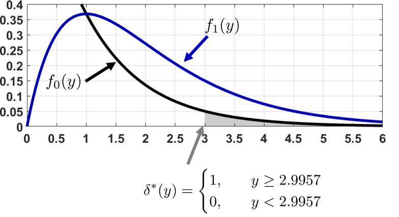
In a telephone system, the waiting time is defined as the inter-arrival time between two consecutive calls. However, it is known that sometimes the waiting time can be mistakenly recorded as the time between three consecutive calls (i.e., by skipping the second one). Since the interarrival time of an independent Poisson process is either an exponential random variable or an Erlang random variable, depending on how many occurrences we are counting, we define the hypotheses

\begin{aligned} f_0(y) = \begin{cases} e^{-y}, &\quad y \ge 0,\\ 0, &\quad y < 0, \end{cases} \quad\mbox{and}\quad f_1(y) = \begin{cases} ye^{-y}, &\quad y \ge 0,\\ 0, &\quad y < 0. \end{cases} \end{aligned}

Suppose we are given one measurement $Y = y$. Find the Neyman-Pearson decision rule for $\alpha = 0.05$.

Solution

The likelihood ratio is

L(y) = \frac{f_1(y)}{f_0(y)} = \frac{ye^{-y}}{e^{-y}} = y, \qquad y \ge 0.

Substituting this into the decision rule, we have

\begin{aligned} \delta^*(y) = \begin{cases} 1, &\qquad L(y) \ge \eta \Longleftrightarrow y \ge \eta,\\ 0, &\qquad L(y) < \eta \Longleftrightarrow y < \eta. \end{cases} \end{aligned}

It remains to determine $\eta$. Inspecting $p_F(\delta)$, we have that

\begin{aligned} \alpha = p_F(\delta^*) &= \int_{L(y)\ge \eta} f_0(y) \;dy \\ &= \int_{y \ge \eta} e^{-y} \;dy = e^{-\eta}. \end{aligned}

Setting $e^{-\eta} = \alpha$, we have that $\eta = -\log \alpha$. Hence, the decision rule is

\begin{aligned} \delta^*(y) = \begin{cases} 1, &\qquad L(y) \ge \eta \Longleftrightarrow y \ge -\log \alpha,\\ 0, &\qquad L(y) < \eta \Longleftrightarrow y < -\log \alpha. \end{cases} \end{aligned}

For $\alpha = 0.05$, we reject the null hypothesis when $y \ge 2.9957$. Figure 9.23 illustrates the hypothesis testing rule.

Remark. This example is instructive in that we have only one measurement $Y = y$. If we have repeated measurements and take the average, then the Central Limit Theorem will kick in. In that case, we can resort to our favorite Gaussian distribution or Student's $t$-distribution instead of dealing with the exponential and the Erlang distributions. However, the example demonstrates the usefulness of Neyman-Pearson, especially when the distributions are complicated.