eBook › Chapter 9 · Confidence and Hypothesis

Section 9.3

Hypothesis Testing

Imagine that you are a vaccine company developing COVID-19 vaccines. You gave the vaccine to 934 patients, and 928 patients have developed antigens. How confident can you be that your vaccine is effective? Questions like this are becoming more common nowadays in situations in which we need to make statistically informed choices between YES and NO. The subject of this section is hypothesis testing — a principled statistical procedure used to evaluate statements that should be accepted or rejected.

9.3.1What is a hypothesis?

A hypothesis is a statement that requires testing by observation to determine whether it is true or false. A few examples:

sep0ex
The coin is unbiased.
Students entering the graduate program have GPA $\ge 3$.
More people like orange juice than lemonade.
Algorithm A performs better than Algorithm B.

As you can see from these examples, a hypothesis is something we can test based on the data. Therefore, being “correct” or “wrong” depends on the statistics we have and the cutoff threshold. Accepting or rejecting a hypothesis does not mean that the statement is correct or wrong, since the truth is unknown. If we accept a hypothesis, we have made a better decision solely based on the statistical evidence. It is possible that tomorrow when you have collected more data we may reject a previously accepted hypothesis.

The procedure for testing whether a hypothesis should be accepted or rejected is known as hypothesis testing. In hypothesis testing, we often have two opposite hypotheses:

sep0ex
$H_0$: Null hypothesis. It is the “status quo”, or the current status.
$H_1$: Alternative hypothesis. It is the alternative to the null hypothesis.

To better understand hypothesis testing, consider a courthouse. By default, any person being prosecuted is assumed to be innocent. The police need to show sufficient evidence in order to prove the person guilty. The null hypothesis is the default assumption. Hypothesis testing asks whether we have strong enough evidence to reject the null hypothesis. If our evidence is not strong enough, we must assume that the null hypothesis is possibly true.

Example 9.6

Suggest a null hypothesis and an alternative hypothesis regarding whether a coin is unbiased.

Solution

: Let $\theta$ be the probability of getting a head.

sep0ex
$H_0$: $\theta = 0.5$, and $H_1$: $\theta > 0.5$. This is a one-sided alternative.
$H_0$: $\theta = 0.5$, and $H_1$: $\theta < 0.5$. This is another one-sided alternative.
$H_0$: $\theta = 0.5$, and $H_1$: $\theta \not= 0.5$. This is a two-sided alternative.

Practice Exercise 9.3

Suggest a null and an alternative hypothesis regarding whether more than 62% of people in the United States use Microsoft Windows.

Solution

: Let $\theta$ be the proportion of people using Microsoft Windows in the United States.

sep0ex
$H_0$: $\theta \ge 0.62$, and $H_1$: $\theta < 0.62$. This is a one-sided alternative.

Practice Exercise 9.4

Suggest a null and an alternative hypothesis regarding whether self-checkout at Walmart is faster than using a cashier.

Solution

: Let $\theta$ be the proportion of people that check out faster with self-checkout.

sep0ex
$H_0$: $\theta \ge 0.5$, and $H_1$: $\theta < 0.5$. This is a one-sided alternative.

9.3.2Critical-value test

In hypothesis testing, there are two major approaches: the critical-value test, and the $p$-value test. The two tests are more or less equivalent. If you reject the null hypothesis using the critical-value test, you will reject the hypothesis using the $p$-value. In this subsection, we will discuss the critical-value test. Let us consider a toy problem:

Suppose that we have a 4-sided die and our goal is to test whether the die is unbiased. To do so, we define the null and the alternative hypotheses as

sep0ex
$H_0$: $\theta = 0.25$, which is our default belief.
$H_1$: $\theta > 0.25$, which is a one-sided alternative.

There is no particular reason for considering the one-sided alternative other than the fact that the calculation is slightly easier. You are welcome to consider the two-sided alternative.

We must obtain data prior to conducting any hypothesis testing. Let's assume that we have thrown the die $N = 1000$ times. We find that “3” appears 290 times (we could just as well have chosen 1, 2, or 4). We let $X_1,\ldots,X_{1000}$ be the $N = 1000$ binary random variables representing whether we have obtained a “3” or not. If the true probability is $\theta = 0.25$, then we will have $\Pb[X_n = 3] = \theta = 0.25$ and $\Pb[X_n \not= 3] = 1-\theta = 0.75$. We know that we cannot access the true probability, so we can only construct an estimator of the probability:

\Thetahat = \frac{1}{N} \sum_{n=1}^N X_n.

In this experiment, we can show that $\Thetahat = 290/1000 = 0.29$.

To make our problem slightly easier, we pretend that we know the variance $\Var[X_n]$. In practice, we certainly do not know $\Var[X_n]$, and so we need to estimate the variance. If we knew the variance, it should be $\Var[X_n] = \theta(1-\theta) = 0.25(1-0.25) = 0.1875$, because $X_n$ is a Bernoulli random variable with a mean $\theta$.

The question asked by hypothesis testing is: How far is “$\Thetahat = 0.29$” from “$\theta = 0.25$”? If the statistic generated by our data, $\Thetahat = 0.29$, is “far” from the hypothesized $\theta = 0.25$, then we need to reject $H_0$ because $H_0$ says that $\theta = 0.25$. However, if there is no strong evidence that $\theta > 0.25$, we will need to assume that $H_0$ may possibly be true. So the key question is what is meant by “far”.

For many problems like this one, it is possible to analyze the PDF of $\Thetahat$. Since $\Thetahat$ is the sample average of a sequence of Bernoulli random variables, it follows that $\Thetahat$ is a binomial (with a scaling constant $1/N$). If $N$ is large enough, e.g., $N \ge 30$, the Central Limit Theorem tells us that $\Thetahat$ is also very close to a Gaussian. Therefore, we can more or less claim that

\Thetahat \sim \text{Gaussian}\left(\theta, \frac{\sigma^2}{N}\right).

With a simple translation and scaling, we can normalize $\Thetahat$ to obtain $\widehat{Z}$:

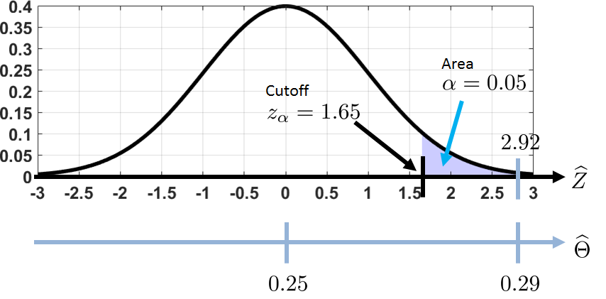
\widehat{Z} = \frac{\Thetahat-\theta}{\sigma/\sqrt{N}} \sim \text{Gaussian}\left(0, 1\right).

Figure 9.10 illustrates the range of values for this problem. There are two axes: the $\Thetahat$-axis (which is the estimator) and the $\widehat{Z}$-axis (which is the normalized variable). The values corresponding to each axis are shown in the figure. For example, $\Thetahat = 0.29$ is equivalent to $\widehat{Z} = 2.92$, and $\Thetahat = 0.25$ is equivalent to $\widehat{Z} = 0$, etc. Therefore, when we ask how far “$\Thetahat = 0.29$” is from “$\theta = 0.25$”, we can map this question from the $\Thetahat$-axis to the $\widehat{Z}$-axis, and ask the relative position of $\widehat{Z}$ from the origin.

On a computer, obtaining these values is quite straightforward. Using MATLAB, finding $\widehat{Z}$ can be done by calling the following commands. The Python code is analogous.

MATLAB

% MATLAB command to estimate the Z_hat value.
    Theta_hat = 0.29;                    % Your estimate
    theta    = 0.25;                     % Your hypothesis
    sigma    = sqrt(theta*(1-theta));    % Known standard deviation
    N        = 1000;                     % Number of samples
    Z_hat    = (Theta_hat - theta)/(sigma/sqrt(N));

Python

# Python command to estimate the Z_hat value
    import numpy as np
    Theta_hat = 0.29                     # Your estimate
    theta     = 0.25                     # Your hypothesis
    N         = 1000                     # Number of samples
    sigma     = np.sqrt(theta*(1-theta)) # Known standard deviation
    Z_hat = (Theta_hat - theta)/(sigma / np.sqrt(N))
    print(Z_hat)

One essential element of hypothesis testing is the cutoff threshold, which is defined through the critical level $\alpha$. It is the area under the curve of the PDF of $\widehat{Z}$. Typically, $\alpha$ is chosen to be a small value, such as $\alpha = 0.05$ (corresponding to a 5% margin). The corresponding cutoff is known as the critical value. It is defined as

z_\alpha = \text{cutoff location where area under the curve is $\alpha$}.

If $\widehat{Z}$ is Gaussian(0,1) and if we are looking at the right-hand tail, it follows that

z_\alpha = \Phi^{-1}\left(1-\alpha\right).

In our example, we find that $z_{0.05} = 1.65$, which is marked in Figure 9.10.

On computers, determining the critical value $z_\alpha$ is straightforward. In MATLAB the command is icdf, and in Python the command is stats.norm.ppf.

MATLAB

% MATLAB code to compute the critical value
    alpha = 0.05;
    z_alpha = icdf('norm', 1-alpha, 0, 1);

Python

# Python code to compute the critical value
    import scipy.stats as stats
    alpha = 0.05
    z_alpha = stats.norm.ppf(1-alpha, 0, 1)

Do we have enough evidence to reject $H_0$ in this example? Of course! The estimated value $\Thetahat = 0.29$ is equivalent to $\widehat{Z} = 2.92$, which is much too far from the cutoff $z_\alpha = 1.65$. In other words, we conclude that at a 5% critical level we have strong evidence to believe that the die is biased. Therefore, we need to reject $H_0$.

This conclusion makes a lot of sense if you think about it carefully. The estimator $\Thetahat = 0.29$ is obtained from $N = 1000$ independent experiments. If we were only conducting $N = 20$ experiments, it might be consistent with the null hypothesis to have $\Thetahat = 0.29$. However, if we have $N =1000$ experiments, having $\Thetahat = 0.29$ does not seem likely when there is no systematic bias. If there is no systematic bias, the estimator $\Thetahat$ should slightly jitter around $\Thetahat = 0.25$, but it is quite unlikely to vary wildly to $\Thetahat = 0.29$. Thus, based on the available statistics, we decide to reject the null hypothesis.

The decision based on comparing the critical value is known as the critical-value test. The idea (for testing a right-hand tail of a Gaussian random variable) is summarized in three steps:

How to conduct a critical-value test

sep0ex
Set a critical value $z_\alpha$. Compute $\widehat{Z} = (\Thetahat-\theta)/(\sigma/\sqrt{N})$.
If $\widehat{Z} \ge z_\alpha$, then reject $H_0$.
If $\widehat{Z} < z_\alpha$, then keep $H_0$.

If you are testing a left-hand tail, you can switch the order of the inequalities.

The critical-value test belongs to a larger family of testing procedures based on decision theory. To give you a preview of the general theory of hypothesis testing, we define a decision rule, a function that maps a realization of the estimator to a binary decision space. In our problem the estimator is $\widehat{Z}$ (or equivalently $\Thetahat$). We denote its realization by $\widehat{z}$. The binary decision space is $\{H_0, \; H_1\}$, corresponding to whether we want to claim $H_0$ or $H_1$. Claiming $H_0$ is equivalent to keeping $H_0$, and claiming $H_1$ is equivalent to rejecting $H_0$. For the critical-value test, the decision rule $\delta(\cdot): \R \rightarrow \{0,1\}$ is given by the equation (for testing a right-hand tail):

\delta(\widehat{z}) = \begin{cases} 1, \quad &\text{if} \;\;\; \widehat{z} \ge z_\alpha, \qquad (\text{claim $H_1$}),\\ 0, \quad &\text{if} \;\;\; \widehat{z} < z_\alpha, \qquad (\text{claim $H_0$}). \end{cases}

Example 9.7

It was found that only 35% of the children in a kindergarten eat broccoli. The teachers conducted a campaign to get more kids to eat broccoli, after which it was found that 390 kids out of 1009 kids reported that they had eaten broccoli. Has the campaign successfully increased the number of kids eating broccoli? Assume that the standard deviation is known.

Solution

We set up the null and the alternative hypothesis.

\begin{aligned} H_0: \;\; \theta = 0.35, \hspace{6ex} H_1: \;\; \theta > 0.35. \end{aligned}

We construct an estimator $\Thetahat = (1/N)\sum_{n=1}^N X_n$, where $X_n$ is Bernoulli with probability $\theta$. Based on $\theta$, $\sigma^2 = \theta(1-\theta) = 0.227$. (Again, in practice we do not know the true variance, but in this problem we pretend that we know it.)

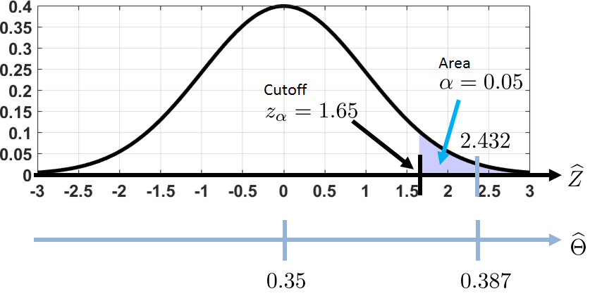
By the Central Limit Theorem, $\Thetahat$ is roughly a Gaussian. We compute the test statistic $\Thetahat = \frac{390}{1009} = 0.387$. Standardization gives $\widehat{Z} = \frac{\Thetahat - \theta}{\sigma/\sqrt{N}} = 2.432$. At a 5% critical level, we have that $z_\alpha = 1.65$. So $\widehat{Z} = 2.432 > 1.65 = z_\alpha$, and hence we need to reject the null hypothesis. Even if we choose a 1% critical level so that $z_\alpha = 2.32$, our estimator $\widehat{Z} = 2.432 > 2.32 = z_\alpha$ will still reject the null hypothesis.

A graphical illustration of this problem is shown in Figure 9.11. It can be seen that $\Thetahat = 0.387$ is actually quite far away from the cutoff 1.65. Thus, we need to reject the null hypothesis.

9.3.3$p$-value test

An alternative to the critical-value test is the $p$-value test. Instead of looking at the cutoff value $z_\alpha$, we inspect the probability of obtaining our observation if $H_0$ is true. To understand how the $p$-value test works, we consider another toy problem.

Suppose that we have two hypotheses about flipping a coin:

sep0ex
$H_0$: $\theta = 0.9$, which is our default belief.
$H_1$: $\theta < 0.9$, which is a one-sided alternative.

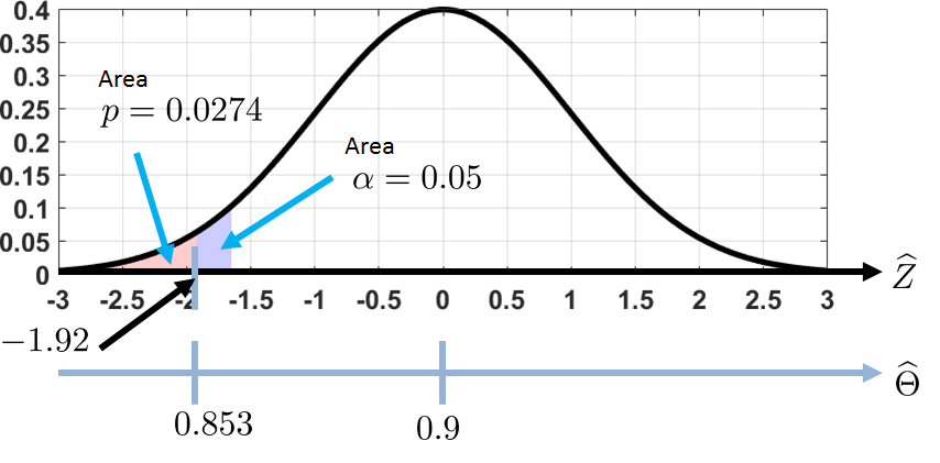
It was found that with $N = 150$ coin flips, the coin landed on heads 128 times. Thus the estimator is $\Thetahat = \frac{128}{150} = 0.853$. Then, by following our previous procedures, we have that

\widehat{Z} = \frac{\Thetahat - \theta}{\sigma/\sqrt{N}} = \frac{0.853-0.9}{\sqrt{\frac{0.9(1-0.9)}{150}}} = -1.92.

At this point we can follow the previous subsection by computing the critical value $z_\alpha$ and making the decision. However, let's take a different route. We want to know what the probability is under the curve if we integrate the PDF of $\widehat{Z}$ from $-\infty$ to $-1.92$. This is easy. Since $\widehat{Z}$ is $\text{Gaussian}(0,1)$, it follows from the CDF of a Gaussian that

\underset{\text{$p$-value}}{\underbrace{\Pb[\widehat{Z} \le -1.92]}} = 0.0274.

Referring to Figure 9.12, the value 0.0274 is the pink area under the curve, which is the PDF of $\widehat{Z}$. Since the area under the curve is less than the critical level $\alpha$ (say 5%), we reject the null hypothesis.

On computers, computing the $p$-value is done using the CDF commands.

MATLAB

% MATLAB code to compute the p-value
    p = cdf('norm', -1.92, 0, 1);

Python

# Python code to compute the p-value
    import scipy.stats as stats
    p = stats.norm.cdf(-1.92,0,1)

In this example, the probability $\Pb[\widehat{Z} \le -1.92]$ is known as the $p$-value. It is the probability of $\widehat{Z} \le z$, under the distribution mandated by the null hypothesis, where $z$ is the (normalized) estimated value based on data. Using our example, $z$ is $-1.92$. By “distribution mandated by the null hypothesis” we mean that the PDF of $\widehat{Z}$ is the PDF that the null hypothesis wants. In the above example the PDF is $\text{Gaussian}(0,1)$, corresponding to $\text{Gaussian}(\theta,\sigma/\sqrt{N})$ for $\widehat{\Theta}$.

More formally, the $p$-value for a left-hand tail test is defined as

p\text{-value}(\widehat{z}) = \Pb[\widehat{Z} \le \widehat{z}],

where $\widehat{z}$ is the random realization of $\widehat{Z}$ estimated from the data. The decision rule based on the $p$-value is (for the left-hand tail):

\delta(\widehat{z}) = \begin{cases} 1, \qquad & \quad \Pb[\widehat{Z} \le \widehat{z}] < \alpha \qquad (\text{claim $H_1$}),\\ 0, \qquad & \quad \Pb[\widehat{Z} \le \widehat{z}] \ge \alpha\qquad (\text{claim $H_0$}). \end{cases}

If the alternative hypothesis is right-handed, then the probability becomes $\Pb[\widehat{Z} \ge \widehat{z}]$ instead.

Relationship between critical-value and $p$-value tests. There is a one-to-one correspondence between the $p$-value and the critical value. In the $p$-value test, if $\widehat{Z}$ is Gaussian, it follows that

\begin{aligned} p\text{-value} = \Pb[\widehat{Z} \le \widehat{z}] = \Phi(\widehat{z}), \end{aligned}

where $\Phi$ is CDF of the standard Gaussian. Taking the inverse, the corresponding $\widehat{z}$ is

\widehat{z} = \Phi^{-1}(p\text{-value}).

In practice, we do not need to take any inverse of the $p$-value to obtain $\widehat{z}$ because it is directly available from the data.

To test the $p$-value, we compare it with the critical level $\alpha$ by checking $$p\text{-value} < \alpha.$$ Taking the inverse of both sides, it follows that the decision rule is equivalent to

\begin{aligned} \underset{\widehat{z}}{\underbrace{\Phi^{-1}(p\text{-value})}} < \underset{z_\alpha}{\underbrace{\Phi^{-1}(\alpha)}}, \end{aligned}

where the quantity on the right-hand side is the critical value $z_\alpha$. Therefore, if the test statistic fails in the $p$-value test, it will also fail in the critical-value test, and vice versa.

What is the difference between the critical-value test and $p$-value test?

sep0ex
Critical-value test: Compare w.r.t. critical value, which is the cutoff on the $Z$-axis.
$p$-value test: Compare w.r.t. $\alpha$, which is the probability.
Both will give you the same statistical conclusion. So it does not matter which one you use.

Example 9.8

We flip a coin for $N = 150$ times and find that 128 are heads. Consider two hypotheses

sep0ex
$H_0$: $\theta = 0.9$, which is our default belief.
$H_1$: $\theta \not= 0.9$, which is a two-sided alternative.

For a critical level of $\alpha = 0.05$, shall we keep or reject $H_0$?

Solution

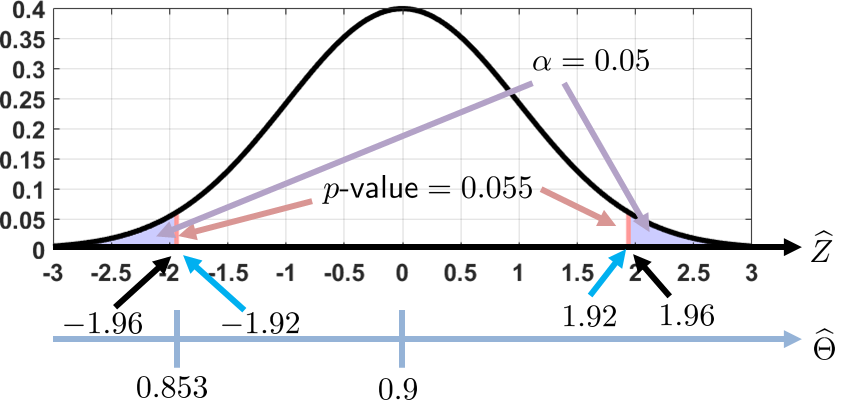
We know that $\Thetahat = 128/150 = 0.853$. The normalized statistic is

\widehat{Z} = \frac{\Thetahat - \theta}{\sigma/\sqrt{N}} = \frac{0.853-0.9}{\sqrt{\frac{0.9(1-0.9)}{150}}} = -1.92.

To compute the $p$-value, we observe that the two-sided test means that we consider the two tails. Thus, we have

\begin{aligned} p\text{-value} &= \Pb[|\widehat{Z}| > 1.92] \\ &= 2 \times \Pb[\widehat{Z} > 1.92] \\ &= 2 \times 0.0274 = 0.055. \end{aligned}

For a critical level of $\alpha = 0.05$, the $p$-value is larger. This means that the probability of obtaining $|Z| > 1.92$ is not extreme enough. Therefore, we do not have sufficient evidence to reject the null hypothesis.

If we take the critical-value test, we will reach the same conclusion. The critical value for $\alpha = 0.05$ is determined by taking the inverse CDF at $1-0.025$, giving

\begin{aligned} z_\alpha = \Phi^{-1}\left(1-\frac{\alpha}{2}\right) = 1.96. \end{aligned}

Since $\widehat{Z} = 1.92$ has not passed this threshold, we conclude that there is not enough evidence to reject the null hypothesis.

**Figure 9.13.** Example of a two-sided test using the $p$-value and the $z_\alpha$-value.

9.3.4$Z$-test and $T$-test

The critical-value test and the $p$-value test are generic tools for hypothesis testing. In this subsection we introduce the $Z$-test and the $T$-test. It is important to understand that the $Z$-test and the $T$-test refer to the distributional assumptions we make about the variance. They define the distribution we use to conduct the test but not the tools. In fact, both the $Z$-test and the $T$-test can be implemented using the critical-value test or the $p$-value test. Figure 9.14 illustrates the hierarchy of the tests.

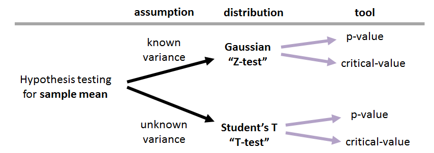
**Figure 9.14.** When conducting a hypothesis test for the sample average, we may or may not know the variance. If we know the variance, we use the Gaussian distribution to conduct either a $p$-value test or a critical-value test. If we do not know the variance, we use Student's $t$-distribution.

The difference between the Gaussian distribution and the $T$ distribution is mainly attributable to the knowledge about the population variance. If the variance is known, the distribution of the estimator (which in our case is the sample average) is Gaussian. If the variance is estimated from the sample, the distribution of the estimator will follow a Student's $t$-distribution.

To introduce the $Z$-test and the $T$-test we consider the following two examples. The first example is a $Z$-test.

Example 9.9

($Z$-test). Suppose we have a Gaussian random variable with unknown mean $\theta$ and a known variance $\sigma = 11.6$. We draw $N = 25$ samples and construct an estimator $\Thetahat = 80.94$. We propose two hypotheses:

sep0ex
$H_0$: $\theta = 85$, which is our default belief.
$H_1$: $\theta < 85$, which is a one-sided alternative.

For a critical level of $\alpha = 0.05$, shall we keep or reject the null hypothesis?

Solution

The test statistic is

\widehat{Z} = \frac{\Thetahat - \theta}{\sigma/\sqrt{N}} = -1.75.

Since the individual samples are assumed to follow a Gaussian, the sample average $\Thetahat$ is also a Gaussian. Hence, $\widehat{Z}$ is distributed according to $\text{Gaussian}(0,1)$.

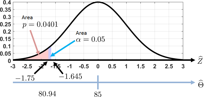
**Figure 9.15.** A one-sided $Z$-test using the $p$-value and the $z_\alpha$-value.

For a critical level of $0.05$, a one-sided critical value is

\begin{aligned} z_\alpha = \Phi^{-1}(\alpha) = -1.645. \end{aligned}

Since $\widehat{Z} = -1.75$, which is more extreme than the critical value, we conclude that we need to reject $H_0$.

If we use the $p$-value test, we have that the $p$-value is

\begin{aligned} \Pb[\widehat{Z} \le -1.75] = \Phi(-1.75) = 0.0401. \end{aligned}

Since the $p$-value is smaller than the critical level $\alpha = 0.05$, it implies that $\widehat{Z} = -1.75$ is more extreme. Hence, we reject $H_0$.

The following example is a $T$-test. In a $T$-test we do not know the population variance but only know the sample variance $\widehat{S}$. Thus the test statistic we use is a $T$ random variable.

Example 9.10

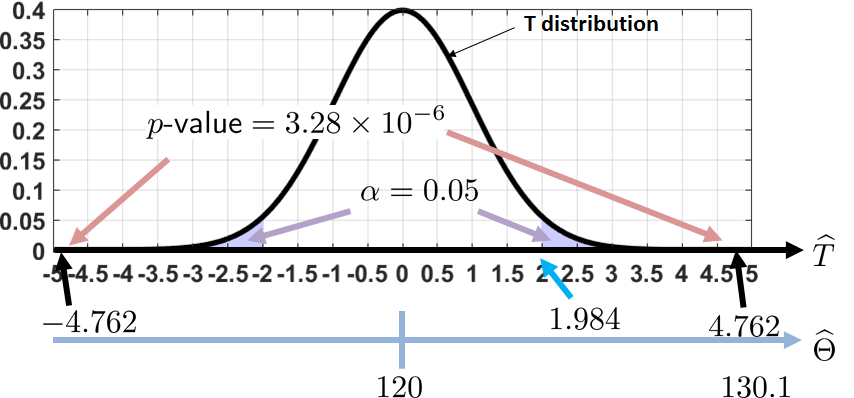
($T$-test). Suppose we have a Gaussian random variable with unknown mean $\theta$ and an unknown variance $\sigma$. We draw $N = 100$ samples and construct an estimator $\Thetahat = 130.1$, with a sample variance $\widehat{S} = 21.21$. We propose two hypotheses:

sep0ex
$H_0$: $\theta = 120$, which is our default belief.
$H_1$: $\theta \not= 120$, which is a two-sided alternative.

For a critical level of $\alpha = 0.05$, shall we keep or reject the null hypothesis?

Solution

The test statistic is

\widehat{T} = \frac{\Thetahat - \theta}{\widehat{S}/\sqrt{N}} = 4.762.

Note that while the sample average $\Thetahat$ is a Gaussian, the test statistic $\widehat{T}$ is distributed according to a $T$ distribution with $N-1$ degrees of freedom. For a critical level of $0.05$, a two-sided critical value is

\begin{aligned} t_\alpha = \Psi_{99}^{-1}\left(1-\frac{\alpha}{2}\right) = 1.984. \end{aligned}

Since $\widehat{T} = 4.762$, which is more extreme than the critical value, we conclude that we need to reject $H_0$.

If we use the $p$-value test, we have that the $p$-value is

\begin{aligned} \Pb[|\widehat{T}| \ge 4.762] &= 2 \times \Pb[\widehat{T} \ge 4.762] \\ &= 6.56 \times 10^{-6}. \end{aligned}

Since the $p$-value is (much) smaller than the critical level $\alpha = 0.05$, it implies that $|\widehat{T}| \ge 4.762$ is quite extreme. Hence, we reject $H_0$.

**Figure 9.16.** A two-sided $T$-test using the $p$-value and the $z_\alpha$-value.

For this example, the MATLAB and Python commands to compute $t_\alpha$ and the $p$-value are

MATLAB

% MATLAB code to compute critical-value and p-value
    t_alpha = icdf('t', 1-0.025, 99);
    p = 1-cdf('t', 4.762, 99);

Python

# Python code to compute critical value and p-value
    import scipy.stats as stats
    t_alpha = stats.t.ppf(1-0.025,99)
    p = 1-stats.t.cdf(4.762,99)

What are the $Z$-test and the $T$-test?

sep0ex
Both are hypothesis tests for the sample averages.
$Z$-test: Assume known variance. Hence, use the Gaussian distribution.
$T$-test: Assume unknown variance. Hence, use the Student's $t$-distribution.

Remark. We are exclusively analyzing the sample average in this section. There are other types of estimators we can analyze. For example, we can discuss the difference between the two means, the ratio of two random variables, etc. If you need tools for these more advanced problems, please refer to the reference section at the end of this chapter.

Hypothesis Testing

9.3.1What is a hypothesis?

9.3.2Critical-value test

9.3.3\(p\)-value test

9.3.4\(Z\)-test and \(T\)-test