eBook › Chapter 9 · Confidence and Hypothesis

Section 9.2

Bootstrapping

When estimating the confidence interval, we focus exclusively on the sample average \(\Thetahat = (1/N)\sum_{n=1}^N X_n\). There are, however, many estimators that are not sample averages. For example, we might be interested in an estimator that estimates the sample median: \(\Thetahat = \text{median}\{X_1,\ldots,X_N\}\). In such cases, the Gaussian-based analysis or the Student's \(t\)-based analysis we just derived would not work.

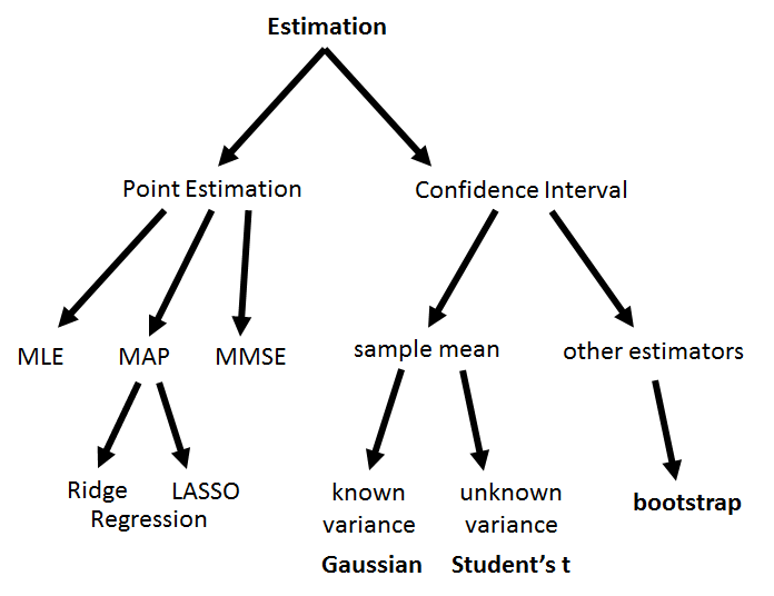
Stepping back a little further, it is important to understand the hierarchy of estimation. Figure 9.8 illustrates a rough breakdown of the various techniques. On the left-hand side of the tree, we have three point estimation methods: MLE, MAP, and MMSE. They are so-called point estimation methods because they are reporting a point — a single value. This stands in contrast to the right-hand side of the tree, in which we report the confidence interval. Note that point estimates and confidence intervals do not conflict with each other. The point estimates are used for the actual engineering solution and the confidence intervals are used to report the confidence about the point estimates. Under the branch of confidence intervals we discussed the sample average. However, if we want to study an estimator that is not the sample average, we need the technique known as the bootstrapping — a method for estimating the confidence interval. Notably, it does not give you a better point estimate.

As we have frequently emphasized, since \(\Thetahat\) is a random variable, it has its own PDF, CDF, mean, variance, etc. The confidence interval introduced in the previous section provides one way to quantify the randomness of \(\Thetahat\). Throughout the derivation of the confidence interval we need to estimate the variance \(\Var(\Thetahat)\). For simple problems such as the sample average, analyzing \(\Var(\Thetahat)\) is not difficult. However, if \(\Thetahat\) is a more complicated statistic, e.g., the median, analyzing \(\Var(\Thetahat)\) may not be as straightforward. Bootstrapping is a technique that is suitable for this purpose.

Why is it difficult to provide a confidence interval for estimators such as the median? A couple of difficulties arise:

sep0ex
Many estimators do not have a simple expression for the variance. For simple estimators such as the sample average \(\Thetahat = (1/N)\sum_{n=1}^N X_n\), the variance is \(\sigma^2/N\). If the estimator is the median \(\Thetahat = \text{median}\{X_1,\ldots,X_N\}\), the variance of \(\Thetahat\) will depend on the underlying distribution of the \(X_n\)'s. If the estimator is something beyond the sample median, the variance of \(\Thetahat\) can be even more complicated to determine. Therefore, techniques such as the Central Limit Theorem do not apply here.
We typically have only one set of data points. We cannot re-collect more i.i.d. samples to estimate the variance of the estimator. Therefore, our only option is to squeeze the information from the data we have been given.

When do we use bootstrapping?

sep0ex
Bootstrapping is a technique to estimate the confidence interval.
We use bootstrapping when the estimator does not have a simple expression for the variance.
Bootstrapping allows us to estimate the variance without re-collecting more data.
Bootstrapping does not improve your point estimates.

9.2.1A brute force approach

Before we discuss the idea of bootstrapping, we need to elaborate on the difficulty of estimating the variance using repeated measurements. Suppose that we somehow have access to the population distribution. Let us denote the CDF of this population distribution by \(F_X\), and the PDF by \(f_X\). By having access to the population distribution we can synthetically generate as many samples \(X_n\)'s as we want. This is certainly hypothetical, but let's assume that it is possible for now.

If we have full access to the population distribution, then we are able to draw \(K\) replicate datasets \(\calX^{(1)},\ldots,\calX^{(K)}\) from \(F_X\):

\begin{aligned} \calX^{(1)} &= \{X_1^{(1)}, \ldots, X_N^{(1)}\} \sim F_X, \\ \calX^{(2)} &= \{X_1^{(2)}, \ldots, X_N^{(2)}\} \sim F_X,\\ &\;\; \vdots \\ \calX^{(K)} &= \{X_1^{(K)}, \ldots, X_N^{(K)}\} \sim F_X. \end{aligned}

Each dataset \(\calX^{(k)}\) contains \(N\) data points, and by virtue of i.i.d. all the samples have the same underlying distribution \(F_X\).

For each dataset we construct an estimator \(\Thetahat = g(\cdot)\) for some function \(g(\cdot)\). The estimator takes the data points of the dataset \(\calX\) and returns a value. Since we have \(K\) datasets, correspondingly we will have \(K\) estimators:

\begin{aligned} \Thetahat^{(1)} &= g(\calX^{(1)}) = g(X_1^{(1)}, \ldots, X_N^{(1)}),\\ \Thetahat^{(2)} &= g(\calX^{(2)}) = g(X_1^{(2)}, \ldots, X_N^{(2)}),\\ &\;\; \vdots \\ \Thetahat^{(K)} &= g(\calX^{(K)}) = g(X_1^{(K)}, \ldots, X_N^{(K)}). \end{aligned}

Note that these estimators \(g(\cdot)\) can be anything. It can be the sample average or it can be the sample median. There is no restriction.

Since we are interested in constructing the confidence interval for \(\Thetahat\), we need to analyze the mean and variance of \(\Thetahat\). The true mean and the estimated mean of \(\Thetahat\) are

\begin{aligned} \mathbb{E}[\Thetahat] &= \text{true mean of } \Thetahat,\\ \mathbb{M}(\Thetahat) &= \text{estimated mean based on } \Thetahat^{(1)},\ldots,\Thetahat^{(K)}\\ &\bydef \frac{1}{K}\sum_{k=1}^K \Thetahat^{(k)} = \frac{1}{K}\sum_{k=1}^K g(\calX^{(k)}), \end{aligned}

respectively. Similarly, the true variance and the estimated variance of \(\Thetahat\) are

\begin{aligned} \text{Var}[\Thetahat] &= \text{true variance of } \Thetahat,\\ \mathbb{V}(\Thetahat) &= \text{estimated variance based on } \Thetahat^{(1)},\ldots,\Thetahat^{(K)} \\ &\bydef \frac{1}{K}\sum_{k=1}^K \left(\Thetahat^{(k)}-\mathbb{M}(\Thetahat)\right)^2 \\ &= \frac{1}{K}\sum_{k=1}^K \left(g(\calX^{(k)})-\mathbb{M}(\Thetahat)\right)^2. \end{aligned}

These two equations should be familiar: Since \(\Thetahat\) is a random variable, and \(\{\Thetahat^{(k)}\}\) are i.i.d. copies of \(\Thetahat\), we can compute the average of \(\Thetahat^{(1)},\ldots,\Thetahat^{(K)}\) and the corresponding variance. As the number of repeated trials \(K\) approaches \(\infty\), the estimated variance \(\mathbb{V}(\Thetahat)\) will converge to \(\Var(\Thetahat)\) according to the law of large numbers.

We can summarize the procedure we have just outlined. To produce an estimate of the variance, we run the algorithm below.

0.953pt

Algorithm 1: Brute force method to generate an estimated variance

0.951pt

sep0ex
Assume: We have access to \(F_X\).
Step 1: Generate datasets \(\calX^{(1)},\ldots,\calX^{(K)}\) from \(F_X\).
Step 2: Compute \(\mathbb{M}(\Thetahat)\) and \(\mathbb{V}(\Thetahat)\) based on the samples.
Output: The estimated variance is \(\mathbb{V}(\Thetahat)\).

0.953pt

The problem, however, is that we only have one dataset \(\calX^{(1)}\). We do not have access to \(\calX^{(2)},\ldots,\calX^{(K)}\), and we do not have access to \(F_X\). Therefore, we are not able to approximate the variance using the above brute force simulation. Bootstrapping is a computational technique to mimic the above simulation process by using the available data in \(\calX^{(1)}\).

9.2.2Bootstrapping

The idea of bootstrapping is illustrated in Figure 9.9. Imagine that we have a population CDF \(F_X\) and PDF \(f_X\). The dataset we have in hand, \(\calX\), is a collection of the random realizations of the random variable \(X\). This dataset \(\calX\) contains \(N\) data points \(\calX = \{X_1,\ldots,X_N\}\).

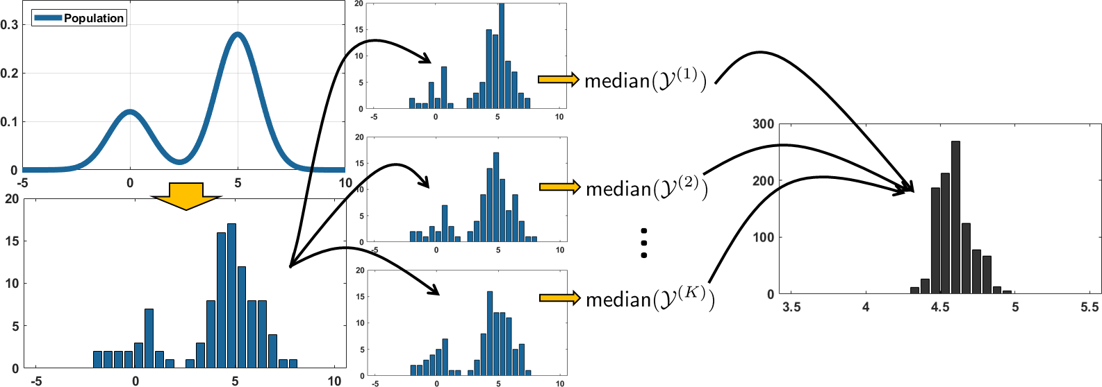
In bootstrapping, we synthesize \(K\) bootstrapped datasets \(\calY^{(1)},\ldots,\calY^{(K)}\), where each bootstrapped dataset \(\calY^{(k)}\) consists of \(N\) samples redrawn from \(\calX\). Essentially, we draw with replacement \(N\) samples from the observed dataset \(\calX\):

\begin{aligned} \calY^{(1)} &= \{Y_1^{(1)},\ldots,Y_N^{(1)}\} = \text{$N$ random samples from $\calX$},\\ &\;\; \vdots\\ \calY^{(K)} &= \{Y_1^{(K)},\ldots,Y_N^{(K)}\} = \text{$N$ random samples from $\calX$}. \end{aligned}

Afterward, we construct our estimator \(\Thetahat\) according to our desired function \(g(\cdot)\). For example, if \(g(\cdot) =\) median, we have

\begin{aligned} \Thetahat^{(1)}_{\text{boot}} &= g(\calY^{(1)}) = \text{median}(\calY^{(1)}),\\ &\;\; \vdots\\ \Thetahat^{(K)}_{\text{boot}} &= g(\calY^{(K)}) = \text{median}(\calY^{(K)}). \end{aligned}

Then, we define the bootstrapped mean and the bootstrapped variance as

\begin{aligned} \mathbb{M}_{\text{boot}}(\Thetahat) &= \frac{1}{K}\sum_{k=1}^K \Thetahat^{(k)}_{\text{boot}},\\ \mathbb{V}_{\text{boot}}(\Thetahat) &= \frac{1}{K}\sum_{k=1}^K \left(\Thetahat^{(k)}_{\text{boot}} - \mathbb{M}_{\text{boot}}(\Thetahat)\right)^2. \end{aligned}

The procedure we have just outlined can be summarized as follows.

0.952pt

Algorithm 2: Bootstrapping to generate an estimated variance

0.951pt

sep0ex
Assume: We do NOT have access to \(F_X\), but we have one dataset \(\calX\).
Step 1: Generate datasets \(\calY^{(1)},\ldots,\calY^{(K)}\) from \(\calX\), by sampling with replacement from \(\calX\).
Step 2: Compute \(\mathbb{M}_{\text{boot}}(\Thetahat)\) and \(\mathbb{V}_{\text{boot}}(\Thetahat)\) based on the samples.
Output: The bootstrapped variance is \(\mathbb{V}_{\text{boot}}(\Thetahat)\).

0.952pt

The only difference between this algorithm and the previous one is that we are not synthesizing data from the population but rather from the observed dataset \(\calX\).

What makes bootstrapping work? The basic principle of bootstrapping is based on three approximations:

\begin{aligned} \Var_F(\Thetahat) & \overset{(a)}{\approx} \mathbb{V}_{\text{full}}(\Thetahat) \\ \rotatebox[origin=c]{90}{$\overset{(b)}{\approx}$} \hspace{4ex} & \\ \Var_{\widehat{F}}(\Thetahat) & \overset{(c)}{\approx} \mathbb{V}_{\text{boot}}(\Thetahat) \end{aligned}

In this set of equations, the ultimate quantity we want to know is \(\Var_F(\Thetahat)\), which is the variance of \(\Thetahat\) under \(F\). (By “under \(F\)” we mean that the variance was found by integrating with respect to the distribution \(F_X\).) However, since we do not have access to \(F\), we have to approximate \(\Var_F(\Thetahat)\) by \(\mathbb{V}_{\text{full}}(\Thetahat)\). \(\mathbb{V}_{\text{full}}(\Thetahat)\) is the sample variance computed from the \(K\) hypothetical datasets \(\calX^{(1)},\ldots,\calX^{(K)}\). We call it “full” because we can generate as many hypothetical datasets as we want. It is marked as the approximation \((a)\) above.

In the bootstrapping world, we approximate the underlying distribution \(F\) by some other distribution \(\widehat{F}\). For example, if \(F\) is the CDF of a Gaussian distribution, we can choose \(\widehat{F}\) to be the finite-sample staircase function approximating \(F\). In our case, we use the observed dataset \(\calX\) to serve as a proxy \(\widehat{F}\) to \(F\). This is the second approximation, marked by \((b)\). Normally, if you have a reasonably large \(\calX\), it is safe to assume that this finite-sample dataset \(\calX\) has a CDF \(\widehat{F}\) that is close to the true CDF \(F\).

The third approximation is to find a numerical estimate \(\Var_{\widehat{F}}(\Thetahat)\) via the simulation procedure we have just outlined. This is essentially the same line of argument for \((a)\) but now applied to the bootstrapping world. We mark this approximation by \((c)\). Its goal is to approximate \(\Var_{\widehat{F}}(\Thetahat)\) via \(\mathbb{V}_{\text{boot}}(\Thetahat)\).

The three approximations have their respective influence on the accuracy of the bootstrapped variance:

How does bootstrapping work?

sep0ex
It is based on three approximations:
\((a)\): A hypothetical approximation. The best we can do is that we have access to \(F\). It is practically impossible to achieve, but it gives us intuition.
\((b)\): Approximate \(F\) by \(\widehat{F}\), where \(\widehat{F}\) is the empirical CDF of the observed data. This is usually the source of error. The approximation error reduces when you use more samples to approximate \(F\).
\((c)\): Approximate the theoretical bootstrapped variance by a finite approximation. This approximation error is usually small because you can generate as many bootstrapped datasets as you want.

One “mysterious” property of bootstrapping is the sampling with replacement scheme used to synthesize the bootstrapped samples. The typical questions are:

sep0ex
(1) Why does sampling from the observed dataset \(\calX\) lead to meaningful bootstrapped datasets \(\calY^{(1)},\ldots,\calY^{(K)}\)? To answer this question we consider the following toy example. Suppose we have a dataset \(\calX\) containing \(N = 20\) samples, as shown below.
MATLAB
```
    X = [0 0 0 0 0 0 1 1 1 1 2 2 2 2 2 2 2 2 2 2]
        
```
This dataset is generated from a random variable \(X\) with a PDF \(\widehat{f}\) having three states: 0 (30%), 1 (20%), 2 (50%). As we draw samples from \(\calX\), the percentage of the states will determine the likelihood of one state being drawn. For example, if we randomly pick a sample \(Y_n\) from \(\calX\), we have a 30% chance that \(Y_n\) is 0, a 20% chance that it is 1, and a 50% chance that it is 2. Therefore, the PDF of \(Y_n\) (the randomly drawn sample from \(\calX\)) will be 0 (30%), 1 (20%), 2 (50%), the same as the original PDF. If you think about this problem more deeply, by “sampling with replacement” we essentially assign each \(X_n\) with an equal probability of \(1/N\). If one of the states is more popular, the individual probabilities will add to form a higher probability mass.
(2) Why can't we do sampling without replacement, aka permutation? We need to understand that sampling without replacement is the same as permuting the data in \(\calX\). By permuting the data in \(\calX\), the simple probability assignments such as \(\Pb[X = 0] = \frac{6}{20}\), \(\Pb[X = 1] = \frac{4}{20}\) and \(\Pb[X = 2] = \frac{10}{20}\) will be destroyed. Moreover, permuting the data does not change the mean and variance of the data because we are only shuffling the order. As far as constructing the confidence interval is concerned, shuffling the order is not useful.

On computers it is easy to generate the bootstrapped dataset, along with its mean and variance. In MATLAB the key step is to call a for loop. Inside the for loop, we draw \(N\) random indices randi from 1 to \(N\) and pick the samples. The estimator Thetahat is then constructed by calling your target estimator function \(g(\cdot)\). In this example the estimator is the median. After the for loop, we compute the mean and variance of \(\Thetahat\). These are the bootstrapped mean and variance, respectively.

MATLAB

% MATLAB code to estimate a bootstrapped variance
    X = [72, 69, 75, 58, 67, 70, 60, 71, 59, 65];
    N = size(X,2);
    K = 1000;
    Thetahat = zeros(1,K);
    for i=1:K                       % repeat K times
        idx = randi(N,[1, N]);      % sampling w/ replacement
        Y = X(idx);
        Thetahat(i) = median(Y);    % estimator
    end
    M = mean(Thetahat)              % bootstrapped mean
    V = var(Thetahat)               % bootstrapped variance

The Python commands are similar. We call np.random.randint to generate random integers and we pick samples according to Y = X[idx]. After generating the bootstrapped dataset, we compute the bootstrap estimators Thetahat.

Python

# Python code to estimate a bootstrapped variance
    import numpy as np
    X = np.array([72, 69, 75, 58, 67, 70, 60, 71, 59, 65])
    N = X.size
    K = 1000
    Thetahat = np.zeros(K)
    for i in range(K):
      idx = np.random.randint(N, size=N)
      Y = X[idx]
      Thetahat[i] = np.median(Y)
    M = np.mean(Thetahat)
    V = np.var(Thetahat)

After we have constructed the bootstrapped variance, we can define the bootstrapped standard error as

\widehat{\text{\textsf{se}}}_{\text{boot}} = \sqrt{\mathbb{V}_{\text{boot}}(\Thetahat)}.

Accordingly we define the bootstrapped confidence interval as

\calI = \big[\Thetahat - z_\alpha \widehat{\text{\textsf{se}}}_{\text{boot}}, \;\; \Thetahat + z_\alpha \widehat{\text{\textsf{se}}}_{\text{boot}}\big],

where \(z_\alpha\) is the critical value of the Gaussian.

The validity of the confidence intervals constructed by bootstrapping is subject to the validity of \(z_\alpha\). If \(\Thetahat\) is roughly a Gaussian, the bootstrapped confidence interval will be reasonably good. If \(\Thetahat\) is not Gaussian, there are advanced methods to replace \(z_\alpha\) with better estimates. This topic is beyond the scope of this book; we refer interested readers to Larry Wasserman, All of Statistics, Springer 2003, Chapter 8.