Probability Mass Function
Random variables are mappings that translate events to numbers. After the translation, we have a set of numbers denoting the states of the random variables. Each state has a different probability of occurring. The probabilities are summarized by a function known as the probability mass function (PMF).
3.2.1Definition of probability mass function
The probability mass function (PMF) of a random variable \(X\) is a function which specifies the probability of obtaining a number \(X(\xi) = x\). We denote a PMF as
The set of all possible states of \(X\) is denoted as \(X(\Omega)\).
Do not get confused by the sample space \(\Omega\) and the set of states \(X(\Omega)\). The sample space \(\Omega\) contains all the possible outcomes of the experiments, whereas \(X(\Omega)\) is the translation by the mapping \(X\). The event \(X = a\) is the set \(X^{-1}(a) \subseteq \Omega\). Therefore, when we say \(\Pb[X = x]\) we really mean \(\Pb[X^{-1}(x)]\).
The probability mass function is a histogram summarizing the probability of each of the states \(X\) takes. Since it is a histogram, a PMF can be easily drawn as a bar chart.
Flip a coin twice. The sample space is \(\Omega = \{\text{HH, HT, TH, TT}\}\). We can assign a random variable \(X\) = number of heads. Therefore, $$X(\text{``HH''})= 2, X(\text{``TH''})= 1, X(\text{``HT''})= 1, X(\text{``TT''})= 0.$$ So the random variable \(X\) takes three states: 0, 1, 2. The PMF is therefore
3.2.2PMF and probability measure
In Chapter 2, we learned that probability is a measure of the size of a set. We introduced a weighting function that weights each of the elements in the set. The PMF is the weighting function for discrete random variables. Two random variables are different when their PMFs are different because they are constructing two different measures.
To illustrate the idea, suppose there are two dice. They each have probability masses as follows.
Let us define two random variables, \(X\) and \(Y\), for the two dice. Then, the PMFs \(p_X\) and \(p_Y\) can be defined as
These two probability mass functions correspond to two different probability measures, let's say \(\mathbb{F}\) and \(\mathbb{G}\). Define the event \(E = \{\text{between 2 and 3}\}\). Then, \(\mathbb{F}(E)\) and \(\mathbb{G}(E)\) will lead to two different results:
Note that even though for some particular events two final results could be the same (e.g., \(1 \le X \le 3\) and \(1 \le Y \le 3\)), the underlying measures are completely different.
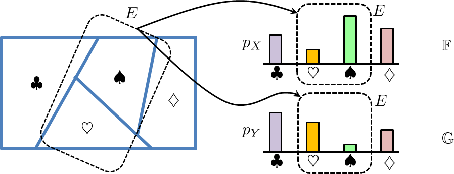
Figure 3.4 shows another example of two different measures \(\mathbb{F}\) and \(\mathbb{G}\) on the same sample space \(\Omega = \{\clubsuit,\diamondsuit,\heartsuit,\spadesuit\}\). Since the PMFs of the two measures are different, even when given the same event \(E\), the resulting probabilities will be different.
Does \(p_X = p_Y\) imply \(X = Y\)? If two random variables \(X\) and \(Y\) have the same PMF, does it mean that the random variables are the same? The answer is no. Consider a random variable with a symmetric PMF, e.g.,
Suppose \(Y = -X\). Then, \(p_Y(-1) = \frac{1}{4}\), \(p_Y(0) = \frac{1}{2}\), and \(p_Y(1) = \frac{1}{4}\), which is the same as \(p_X\). However, \(X\) and \(Y\) are two different random variables. If the sample space is \(\{\clubsuit,\diamondsuit,\heartsuit\}\), we can define the mappings \(X(\cdot)\) and \(Y(\cdot)\) as
Therefore, when we say \(p_X(-1) = \frac{1}{4}\), the underlying event is \(\clubsuit\). But when we say \(p_Y(-1) = \frac{1}{4}\), the underlying event is \(\heartsuit\). The two random variables are different, although their PMFs have exactly the same shape.
3.2.3Normalization property
Here we must mention one important property of a probability mass function. This property is known as the normalization property, which is a useful tool for a sanity check.
A PMF should satisfy the condition that
Proof. The proof follows directly from Axiom II, which states that \(\Pb[\Omega] = 1\). Since \(x\) covers all numerical values \(X\) can take, and since each \(x\) is distinct, by Axiom III we have
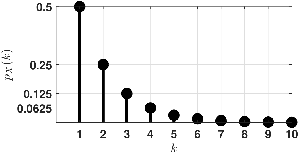
Let \(p_X(k) = c \left(\frac{1}{2}\right)^k\), where \(k = 1,2,\ldots\). Find \(c\).
Since \(\sum_{k \in X(\Omega)} p_X(k) = 1\), we must have $$\sum_{k = 1}^{\infty} c \; \left(\frac{1}{2}\right)^k = 1.$$ Evaluating the geometric series on the left-hand side, we can show that
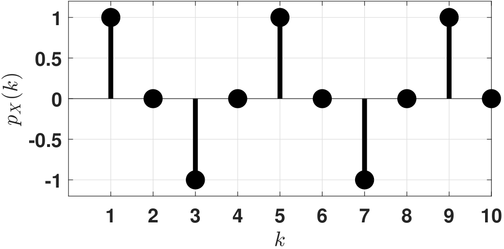
Let \(p_X(k) = c \cdot \sin \left( \frac{\pi}{2} k \right)\), where \(k = 1,2,\ldots\). Find \(c\).
The reader might be tempted to sum \(p_X(k)\) over all the possible \(k\)'s:
However, a more careful inspection reveals that \(p_X(k)\) is actually negative when \(k = 3, 7, 11, \ldots\). This cannot happen because a probability mass function must be non-negative. Therefore, the problem is not defined, and so there is no solution.
3.2.4PMF versus histogram
PMFs are closely related to histograms. A histogram is a plot that shows the frequency of a state. As we see in Figure 3.5, the \(x\)-axis is a collection of states, whereas the \(y\)-axis is the frequency. So a PMF is indeed a histogram.
Viewing a PMF as a histogram can help us understand a random variable. For better or worse, treating a random variable as a histogram could help you differentiate a random variable from a variable. An ordinary variable only has one state, but a random variable has multiple states. At any particular instant, we do not know which state will show up before our observation. However, we do know the probability. For example, in the coin-flip example, while we do not know whether we will get “HH,” we know that the chance of getting “HH” is 1/4. Of course, having a probability of 1/4 does not mean that we will get “HH” once every four trials. It only means that if we run an infinite number of experiments, then 1/4 of the experiments will give us “HH.”
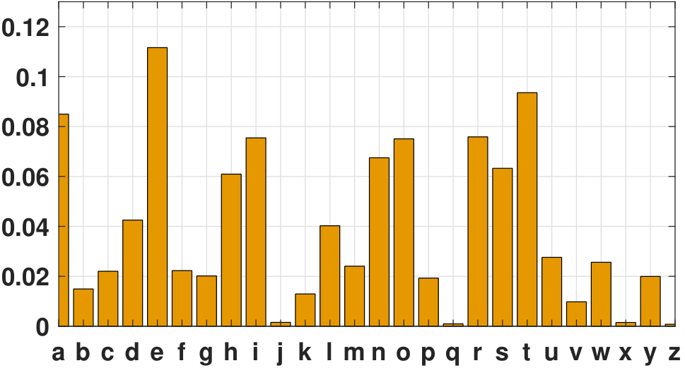
The linkage between PMF and histogram can be quite practical. For example, while we do not know the true underlying distribution of the 26 letters of the English alphabet, we can collect a large number of words and plot the histogram. The example below illustrates how we can empirically define a random variable from the data.
There are 26 English letters, but the frequencies of the letters in writing are different. If we define a random variable \(X\) as a letter we randomly draw from an English text, we can think of \(X\) as an object with 26 different states. The mapping associated with the random variable is straightforward: \(X(\text{``a''}) = 1\), \(X(\text{``b''}) = 2\), etc. The probability of landing on a particular state approximately follows a histogram shown in Figure 3.6. The histogram provides meaningful values of the probabilities, e.g., \(p_X(1) = 0.0847\), \(p_X(2) = 0.0149\), etc. The true probability of the states may not be exactly these values. However, when we have enough samples, we generally expect the histogram to approach the theoretical PMF. The MATLAB and Python codes used to generate this histogram are shown below.
% MATLAB code to generate the histogram
    load(`ch3_data_English');
    bar(f/100,`FaceColor',[0.9,0.6,0.0]);
    xticklabels({`a',`b',`c',`d',`e',`f',`g',`h',`i',`j',`k',`l',...
        `m',`n',`o',`p',`q',`r',`s',`t',`u',`v',`w',`x',`y',`z'});
    xticks(1:26);
    yticks(0:0.02:0.2);
axis([1 26 0 0.13]);# Python code to generate the histogram
import numpy as np
import matplotlib.pyplot as plt
f = np.loadtxt(`./ch3_data_english.txt')
n = np.arange(26)
plt.bar(n, f/100)
ntag = [`a',`b',`c',`d',`e',`f',`g',`h',`i',`j',`k',`l',`m',...
`n',`o',`p',`q',`r',`s',`t',`u',`v',`w',`x',`y',`z']
plt.xticks(n, ntag)PMF = ideal histograms
If a random variable is more or less a histogram, why is the PMF such an important concept? The answer to this question has two parts. The first part is that the histogram generated from a dataset is always an empirical histogram, so-called because the dataset comes from observation or experience rather than theory. Thus the histograms may vary slightly every time we collect a dataset.
As we increase the number of data points in a dataset, the histogram will eventually converge to an ideal histogram, or a distribution. For example, counting the number of heads in 100 coin flips will fluctuate more in percentage terms than counting the heads in 10 million coin flips. The latter will almost certainly have a histogram that is closer to a 50–50 distribution. Therefore, the “histogram” generated by a random variable can be considered the ultimate histogram or the limiting histogram of the experiment.
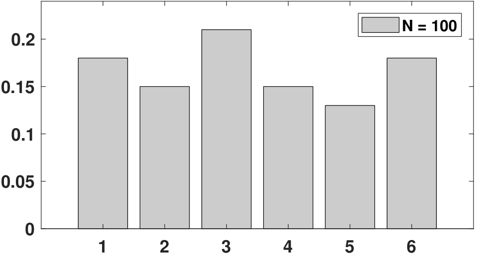
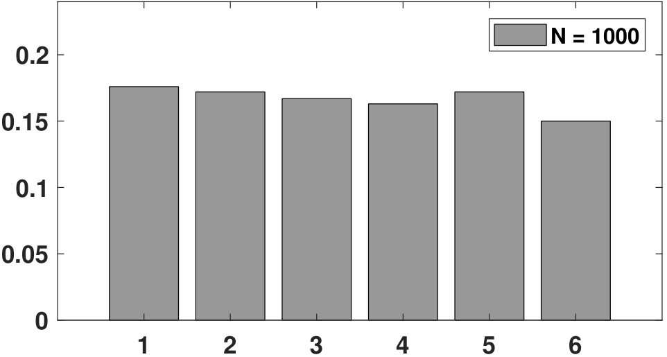
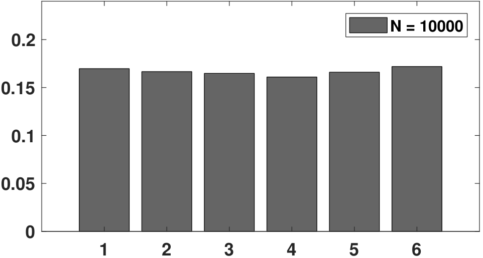
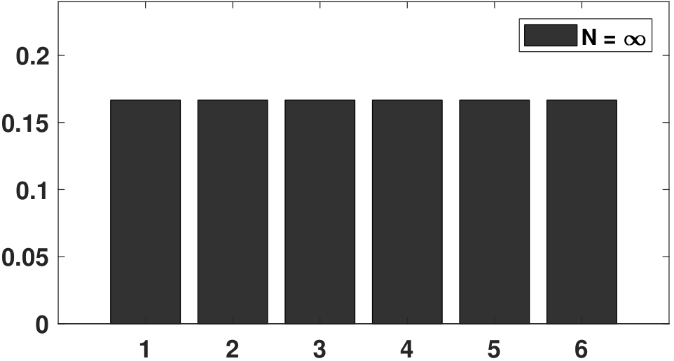
To help you visualize the difference between a PMF and a histogram, we show in Figure 3.7 an experiment in which a die is thrown \(N\) times. Assuming that the die is fair, the PMF is simply \(p_X(k) = 1/6\) for \(k = 1,\ldots,6\), which is a uniform distribution across the 6 states. Now, we can throw the die many times. As \(N\) increases, we observe that the histogram becomes more like the PMF. You can imagine that when \(N\) goes to infinity, the histogram will eventually become the PMF. Therefore, when given a dataset, one way to think of it is to treat the data as random realizations drawn from a certain PMF. The more data points you have, the closer the histogram will become to the PMF.
The MATLAB and Python codes used to generate Figure 3.7 are shown below. The two commands we use here are randi (in MATLAB), which generates random integer numbers, and hist, which computes the heights and bin centers of a histogram. In Python, the corresponding commands are np.random.randint and plt.hist. Note that because of the different indexing schemes in MATLAB and Python, we offset the maximum index in np.random.randint to 7 instead of 6. Also, we shift the \(x\)-axes so that the bars are centered at the integers.
% MATLAB code to generate the histogram
    x = [1 2 3 4 5 6];
    q = randi(6,100,1);
    figure;
    [num,val] = hist(q,x-0.5);
    bar(num/100,`FaceColor',[0.8, 0.8,0.8]);
axis([0 7 0 0.24]);# Python code to generate the histogram
import numpy as np
import matplotlib.pyplot as plt
q = np.random.randint(7,size=100)
plt.hist(q+0.5,bins=6)This generative perspective is illustrated in Figure 3.8. We assume that the underlying latent random variable has some PMF that can be described by a few parameters, e.g., the mean and variance. Given the data points, if we can infer these parameters, we might retrieve the entire PMF (up to the uncertainty level intrinsic to the dataset). We refer to this inverse process as statistical inference.
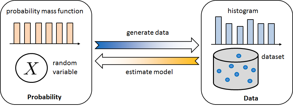
Returning to the question of why we need to understand the PMFs, the second part of the answer is the difference between synthesis and analysis. In synthesis, we start with a known random variable and generate samples according to the PMF underlying the random variable. For example, on a computer, we often start with a Gaussian random variable and generate random numbers according to the histogram specified by the Gaussian random variable. Synthesis is useful because we can predict what will happen. We can, for example, create millions of training samples to train a deep neural network. We can also evaluate algorithms used to estimate statistical quantities such as mean, variance, moments, etc., because the synthesis approach provides us with ground truth. In supervised learning scenarios, synthesis is vital to ensuring sufficient training data.
The other direction of synthesis is analysis. The goal is to start with a dataset and deduce the statistical properties of the dataset. For example, suppose we want to know whether the underlying model is indeed a Gaussian model. If we know that it is a Gaussian (or if we choose to use a Gaussian), we want to know the parameters that define this Gaussian. The analysis direction addresses this model selection and parameter estimation problem. Moving forward, once we know the model and the parameters, we can make a prediction or do recovery, both of which are ubiquitous in machine learning.
We summarize our discussions below, which is Key Concept 2 of this chapter.
PMFs are the ideal histograms of random variables.
3.2.5Estimating histograms from real data
The following discussions about histogram estimation can be skipped if it is your first time reading the book.
If you have a dataset, how would you plot the histogram? Certainly, if you have access to MATLAB or Python, you can call standard functions such as hist (in MATLAB) or np.histogram (in Python). However, when plotting a histogram, you need to specify the number of bins (or equivalently the width of bins). If you use larger bins, then you will have fewer bins with many elements in each bin. Conversely, if the bin width is too small, you may not have enough samples to fill the histogram. Figure 3.9 illustrates two histograms in which the bins are respectively too large and too small.
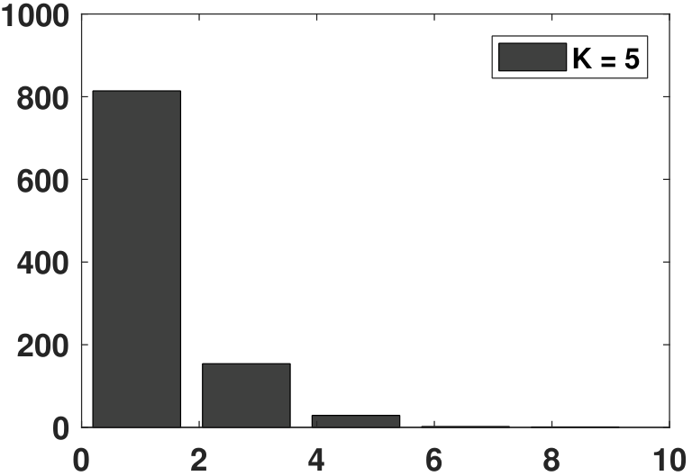
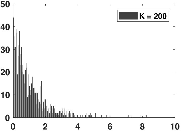
The MATLAB and Python codes used to generate Figure 3.9 are shown below. Note that here we are using an exponential random variable (to be discussed in Chapter 4). In MATLAB, calling an exponential random variable is done using exprnd, whereas in Python the command is np.random.exponential. For this experiment, we can specify the number of bins \(k\), which can be set to \(k=200\) or \(k=5\). To suppress the Python output of the array, we can add a semicolon ;. A final note is that lambda is a reserved variable in Python. Use something else.
% MATLAB code used to generate the plots
    lambda = 1;
    k      = 1000;
    X      = exprnd(1/lambda,[k,1]);
    [num,val] = hist(X,200);
bar(val,num,`FaceColor',[1, 0.5,0.5]);# Python code used to generate the plots
import numpy as np
import matplotlib.pyplot as plt
lambd = 1
k = 1000
X = np.random.exponential(1/lambd, size=k)
plt.hist(X,bins=200);In statistics, there are various rules to determine the bin width of a histogram. We mention a few of them here. Let \(K\) be the number of bins and \(N\) the number of samples.
- sep0em
- Square-root: \(K = \sqrt{N}\)
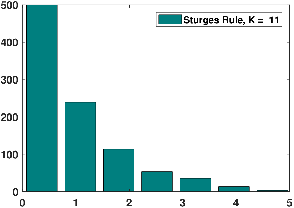
- Sturges' formula: \(K = \log_2 N + 1\).
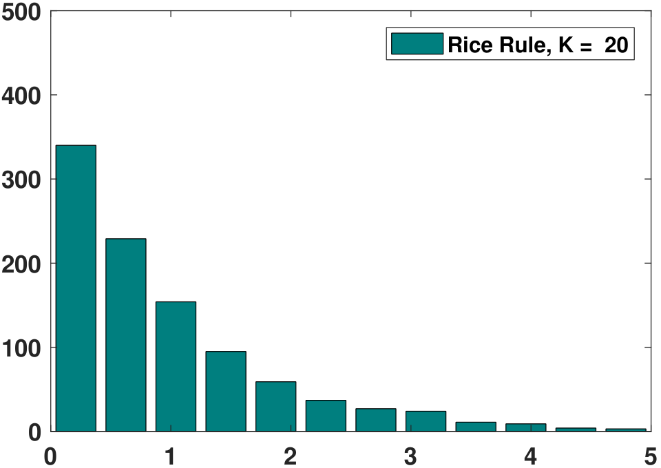
- Rice Rule: \(K = 2\sqrt[3]{N}\)
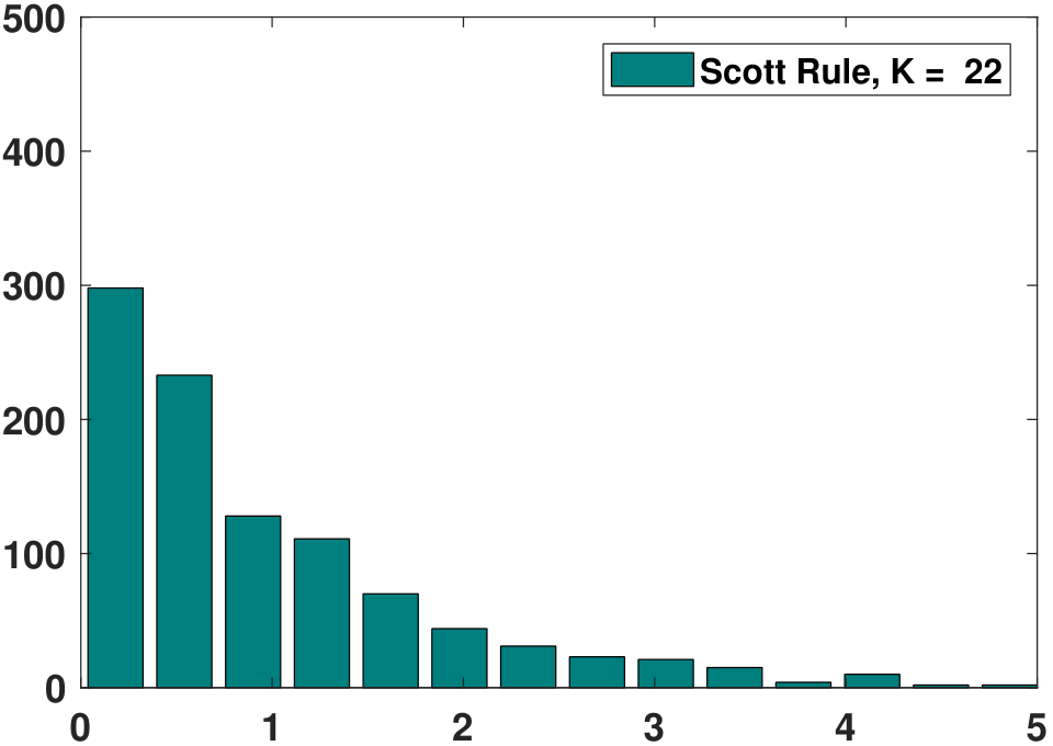
- Scott's normal reference rule: \(K = \frac{\max X - \min X}{h}\), where \(h = \frac{3.5\sqrt{\Var[X]}}{\sqrt[3]{N}}\) is the bin width.
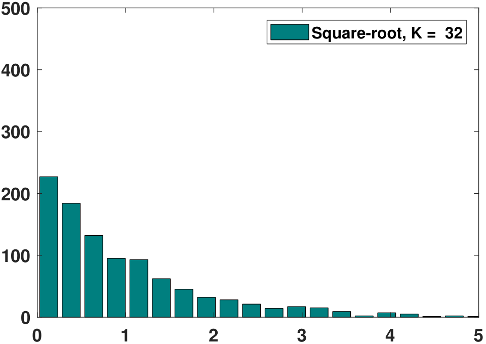
For the example data shown in Figure 3.9, the histograms obtained using the above rules are given in Figure 3.10. As you can see, different rules have different suggested bin widths. Some are more conservative, e.g., using fewer bins, whereas some are less conservative. In any case, the suggested bin widths do seem to provide better histograms than the original ones in Figure 3.9. However, no bin width is the best for all purposes.
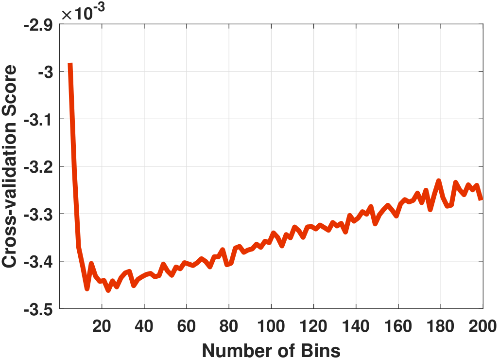
Beyond these predefined rules, there are also algorithmic tools to determine the bin width. One such tool is known as cross-validation. Cross-validation means defining some kind of cross-validation score that measures the statistical risk associated with the histogram. A histogram having a lower score has a lower risk, and thus it is a better histogram. Note that the word “better” is relative to the optimality criteria associated with the cross-validation score. If you do not agree with our cross-validation score, our optimal bin width is not necessarily the one you want. In this case, you need to specify your optimality criteria.
Theoretically, deriving a meaningful cross-validation score is beyond the scope of this book. However, it is still possible to understand the principle. Let \(h\) be the bin width of the histogram, \(K\) the number of bins, and \(N\) the number of samples. Given a dataset, we follow this procedure:
- sep0em
- Step 1: Choose a bin width \(h\).
- Step 2: Construct a histogram from the data, using the bin width \(h\). The histogram will have the empirical PMF values \(\widehat{p}_1,\widehat{p}_2,\ldots,\widehat{p}_K\), which are the heights of the histograms normalized so that the sum is 1.
Step 3: Compute the cross-validation score (see Wasserman, All of Statistics, Section 20.2):
$$J(h) = \frac{2}{(N-1)h} - \frac{N+1}{(N-1)h}\left(\widehat{p}_1^2+\widehat{p}_2^2+\cdots+\widehat{p}_K^2\right)$$- Repeat Steps 1, 2, 3, until we find an \(h\) that minimizes \(J(h)\).
Note that when we use a different \(h\), the PMF values \(\widehat{p}_1,\widehat{p}_2,\ldots,\widehat{p}_K\) will change, and the number of bins \(K\) will also change. Therefore, when changing \(h\), we are changing not only the terms in \(J(h)\) that explicitly contain \(h\) but also terms that are implicitly influenced.
For the dataset we showed in Figure 3.9, the cross-validation score \(J(h)\) is shown in Figure 3.11. We can see that although the curve is noisy, there is indeed a reasonably clear minimum happening around \(20 \le K \le 30\), which is consistent with some of the rules.
The MATLAB and Python codes we used to generate Figure 3.11 are shown below. The key step is to implement Eq. (3.4) inside a for-loop, where the loop goes through the range of bins we are interested in. To obtain the PMF values \(\widehat{p}_1,\ldots,\widehat{p}_K\), we call hist in MATLAB and np.histogram in Python. The bin width h is the number of samples n divided by the number of bins m.
% MATLAB code to perform the cross validation
    lambda = 1;
    n = 1000;
    X = exprnd(1/lambda,[n,1]);
    m = 6:200;
    J = zeros(1,195);
    for i=1:195
        [num,binc] = hist(X,m(i));
        h = n/m(i);
        J(i) = 2/((n-1)*h)-((n+1)/((n-1)*h))*sum( (num/n).^2 );
    end
plot(m,J,`LineWidth',4,`Color',[0.9,0.2,0.0]);# Python code to perform the cross validation
import numpy as np
import matplotlib.pyplot as plt
lambd = 1
n = 1000
X = np.random.exponential(1/lambd, size=n)
m = np.arange(5,200)
J = np.zeros((195))
for i in range(0,195):
hist,bins = np.histogram(X,bins=m[i])
h = n/m[i]
J[i] = 2/((n-1)*h)-((n+1)/((n-1)*h))*np.sum((hist/n)**2)
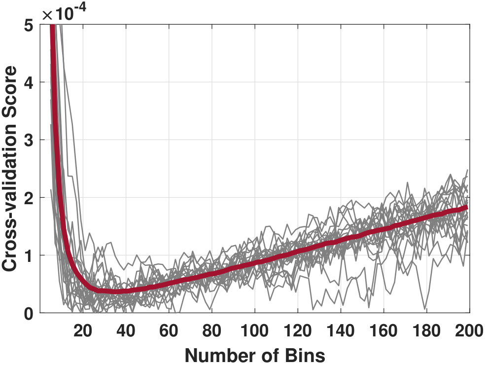
plt.plot(m,J);In Figure 3.11(b), we show another set of curves from the same experiment. The difference here is that we assume access to the true generative model so that we can generate many datasets from the same distribution. In this experiment we generated \(T = 1000\) datasets. We compute the cross-validation score \(J(h)\) for each of the datasets, yielding \(T\) score functions \(J^{(1)}(h), \ldots,J^{(T)}(h)\). We subtract the minimum because different realizations have different offsets. Then we compute the average:
This gives us a smooth red curve as shown in Figure 3.11(b). The minimum appears to be at \(K = 25\). This is the optimal \(K\), concerning the cross-validation score, averaged over all datasets.
All rules, including cross-validation, are based on optimizing for a certain objective. Your objective could be different from our objective, and so our optimum is not necessarily your optimum. Therefore, cross-validation may not be the best. It depends on your problem.
End of the discussion.