Cumulative Distribution Functions (Discrete)

While the probability mass function (PMF) provides a complete characterization of a discrete random variable, the PMFs themselves are technically not “functions” because the impulses in the histogram are essentially delta functions. More formally, a PMF $p_X(k)$ should actually be written as

p_X(x) = \sum_{k \in X(\Omega)} \underset{\text{PMF values}}{\underbrace{ \quad p_X(k) \quad}} \cdot \underset{\text{delta function}}{\underbrace{ \quad \delta(x - k) \quad }}.

This is a train of delta functions, where the height is specified by the probability mass $p_X(k)$. For example, a random variable with PMF values

\begin{aligned} p_X(0) = \frac{1}{4}, \;\; p_X(1) = \frac{1}{2}, \;\; p_X(2) = \frac{1}{4} \end{aligned}

will be expressed as

p_X(x) = \frac{1}{4}\delta(x) + \frac{1}{2}\delta(x-1) + \frac{1}{4}\delta(x-2).

Since delta functions need to be integrated to generate values, the typical things we want to do, e.g., integration and differentiation, are not as straightforward in the sense of Riemann-Stieltjes.

The way to handle the unfriendliness of the delta functions is to consider mild modifications of the PMF. This notion of “cumulative” distribution functions will allow us to resolve the delta function problems. We will defer the technical details to the next chapter. For the time being, we will briefly introduce the idea to prepare you for the technical discussion later.

3.3.1Definition of the cumulative distribution function

Definition 3.3

Let $X$ be a discrete random variable with $\Omega = \{x_1,x_2,\ldots\}$. The cumulative distribution function (CDF) of $X$ is

F_X(x_k) \bydef \Pb[X \le x_k] = \sum_{\ell = 1}^{k} p_X(x_{\ell}).

If $\Omega = \{\ldots, -1, 0, 1, 2, \ldots \}$, then the CDF of $X$ is

F_X(k) \bydef \Pb[X \le k] = \sum_{\ell = -\infty}^{k} p_X(\ell).

A CDF is essentially the cumulative sum of a PMF from $-\infty$ to $x$, where the variable $\ell$ in the sum is a dummy variable.

Example 3.7

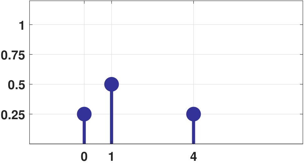
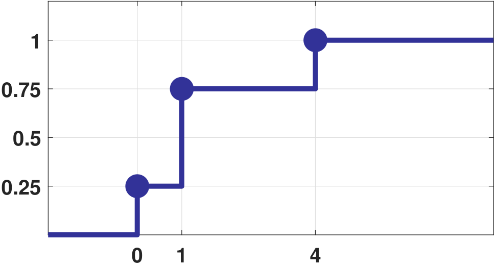
Consider a random variable $X$ with PMF $p_X(0) = \frac{1}{4}$, $p_X(1) = \frac{1}{2}$ and $p_X(4) = \frac{1}{4}$. The CDF of $X$ can be computed as

\begin{aligned} F_X(0) &= \Pb[X \le 0] = p_X(0) = \frac{1}{4}, \\ F_X(1) &= \Pb[X \le 1] = p_X(0) + p_X(1) = \frac{3}{4},\\ F_X(4) &= \Pb[X \le 4] = p_X(0) + p_X(1) + p_X(4) = 1. \end{aligned}

As shown in Figure 3.12, the CDF of a discrete random variable is a staircase function.

**Figure 3.12.** Illustration of a PMF and a CDF.

The MATLAB code and the Python code used to generate Figure 3.12 are shown below. The CDF is computed using the command cumsum in MATLAB and np.cumsum in Python.

MATLAB

% MATLAB code to generate a PMF and a CDF
    p = [0.25 0.5 0.25];
    x = [0 1 4];
    F = cumsum(p);
    
    figure(1);
    stem(x,p,`.',`LineWidth',4,`MarkerSize',50);
    figure(2);
    stairs([-4 x 10],[0 F 1],`.-',`LineWidth',4,`MarkerSize',50);

Python

# Python code to generate a PMF and a CDF
    import numpy as np
    import matplotlib.pyplot as plt
    p = np.array([0.25, 0.5, 0.25])
    x = np.array([0, 1, 4])
    F = np.cumsum(p)
    
    plt.stem(x,p,use_line_collection=True); plt.show()
    plt.step(x,F); plt.show()

Why is CDF a better-defined function than PMF? There are technical reasons associated with whether a function is integrable. Without going into the details of these discussions, a short answer is that delta functions are defined through integrations; they are not functions. A delta function is defined as a function such that $\delta(x)=0$ everywhere except at $x=0$, and $\int_{\Omega} \delta (x) \;dx = 1$. On the other hand, a staircase function is always well-defined. The discontinuous points of a staircase can be well defined if we specify the gap between two consecutive steps. For example, in Figure 3.12, as soon as we specify the gap $1/4$, $1/2$, and $1/4$, the staircase function is completely defined.

Example 3.8

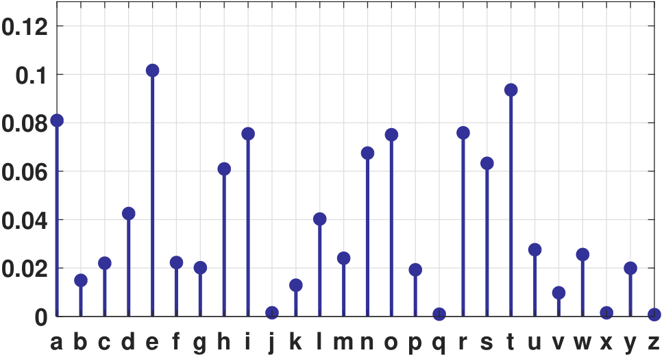
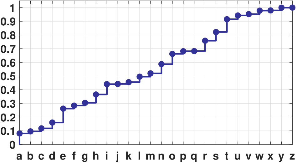
Figure 3.13 shows the empirical histogram of the English letters and the corresponding empirical CDF. We want to differentiate PMF versus histogram and CDF versus empirical CDF. The empirical CDF is the CDF computed from a finite dataset.

**Figure 3.13.** PMF and a CDF of the frequency of English letters.

3.3.2Properties of the CDF

We observe from the example in Figure 3.12 that a CDF has several properties. First, being a staircase function, the CDF is non-decreasing. It can stay constant for a while, but it never drops. Second, the minimum value of a CDF is 0, whereas the maximum value is 1. It is 0 for any value that is smaller than the first state; it is 1 for any value that is larger than the last state. Third, the gap at each jump is exactly the probability mass at that state. Let us summarize these observations in the following theorem.

Theorem 3.2

If $X$ is a discrete random variable, then the CDF of $X$ has the following properties:

(i) The CDF is a sequence of increasing unit steps.
(ii) The maximum of the CDF is when $x = \infty$: $F_X(+\infty) = 1$.
(iii) The minimum of the CDF is when $x = -\infty$: $F_X(-\infty) = 0$.
(iv) The unit steps have jumps at positions where $p_X(x) > 0$.

Proof. Statement (i) can be seen from the summation

\begin{aligned} F_X(x) = \sum_{x' \le x} p_X(x'). \end{aligned}

Since the probability mass function is non-negative, the value of $F_X$ is larger when the value of the argument is larger. That is, $x \le y$ implies $F_X(x) \le F_X(y)$. The second statement (ii) is true because the summation includes all possible states. So we have

\begin{aligned} F_X(+\infty) = \sum_{x' = -\infty}^{\infty} p_X(x') = 1. \end{aligned}

Similarly, for the third statement (iii), $$F_X(-\infty) = \sum_{x' \le -\infty} p_X(x').$$ The summation is taken over an empty set, and so $F_X(-\infty) = 0$. Statement (iv) is true because the cumulative sum changes only when there is a non-zero mass in the PMF.

■

As we can see in the proof, the basic argument of the CDF is the cumulative sum of the PMF. By definition, a cumulative sum always adds mass. This is why the CDF is always increasing, has 0 at $-\infty$, and has 1 at $+\infty$. This last statement deserves more attention. It implies that the unit step always has a solid dot on the left-hand side and an empty dot on the right-hand side, because when the CDF jumps, the final value is specified by the “$\le$” sign in Eq. (3.6). The technical term for this property is right-continuous.

3.3.3Converting between PMF and CDF

Theorem 3.3

If $X$ is a discrete random variable, then the PMF of $X$ can be obtained from the CDF by

p_X(x_k) = F_X(x_k) - F_X(x_{k-1}),

where we assumed that $X$ has a countable set of states $\{x_1,x_2,\ldots\}$. If the sample space of the random variable $X$ contains integers from $-\infty$ to $+\infty$, then the PMF can be defined as

$$p_X(k) = F_X(k) - F_X(k-1).$$

Example 3.9

Continuing with the example in Figure 3.12, if we are given the CDF

\begin{aligned} F_X(0) = \frac{1}{4}, \quad\quad F_X(1) = \frac{3}{4}, \quad\quad F_X(4) = 1, \end{aligned}

how do we find the PMF? We know that the PMF will have non-negative values only at $x = 0, 1, 4$. For each of these $x$, we can show that

\begin{aligned} p_X(0) &= F_X(0) - F_X(-\infty) = \frac{1}{4} - 0 = \frac{1}{4},\\ p_X(1) &= F_X(1) - F_X(0) = \frac{3}{4} - \frac{1}{4}= \frac{1}{2},\\ p_X(4) &= F_X(4) - F_X(1) = 1 - \frac{3}{4} = \frac{1}{4}. \end{aligned}