Common Discrete Random Variables
In the previous sections, we have conveyed three key concepts: one about the random variable, one about the PMF, and one about the mean. The next step is to introduce a few commonly used discrete random variables so that you have something concrete in your “toolbox.” As we have mentioned before, these predefined random variables should be studied from a synthesis perspective (sometimes called generative). The plan for this section is to introduce several models, derive their theoretical properties, and discuss examples.
Note that some extra effort will be required to understand the origins of the random variables. The origins of random variables are usually overlooked, but they are more important than the equations. For example, we will shortly discuss the Poisson random variable and its PMF \(p_X(k) = \frac{\lambda^ke^{-\lambda}}{k!}\). Why is the Poisson random variable defined in this way? If you know how the Poisson PMF was originally derived, you will understand the assumptions made during the derivation. Consequently, you will know why Poisson is a good model for internet traffic, recommendation scores, and image sensors for computer vision applications. You will also know under what situation the Poisson model will fail. Understanding the physics behind the probability models is the focus of this section.
3.5.1Bernoulli random variable
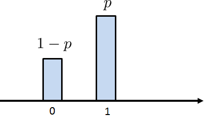
We start discussing the simplest random variable, namely the Bernoulli random variable. A Bernoulli random variable is a coin-flip random variable. The random variable has two states: either 1 or 0. The probability of getting 1 is \(p\), and the probability of getting 0 is \(1-p\). See Figure 3.21 for an illustration. Bernoulli random variables are useful for all kinds of binary-state events: coin flip (H or T), binary bit (1 or 0), true or false, yes or no, present or absent, Democrat or Republican, etc.
To make these notions more precise, we define a Bernoulli random variable as follows.
Let \(X\) be a Bernoulli random variable. Then, the PMF of \(X\) is
where \(0 < p < 1\) is called the Bernoulli parameter. We write $$X \sim \mathrm{Bernoulli}(p)$$ to say that \(X\) is drawn from a Bernoulli distribution with a parameter \(p\).
In this definition, the parameter \(p\) controls the probability of obtaining 1. In a coin-flip event, \(p\) is usually \(\tfrac{1}{2}\), meaning that the coin is fair. However, for biased coins \(p\) is not necessarily \(\tfrac{1}{2}\). For other situations such as binary bits (0 or 1), the probability of obtaining 1 could be very different from the probability of obtaining 0.
In MATLAB and Python, generating Bernoulli random variables can be done by calling the binomial random number generator np.random.binomial (Python) and binornd (MATLAB). When the parameter n is equal to 1, the binomial random variable is equivalent to a Bernoulli random variable. The MATLAB and Python codes to synthesize a Bernoulli random variable are shown below.
% MATLAB code to generate 1000 Bernoulli random variables
    p = 0.5;
    n = 1;
    X = binornd(n,p,[1000,1]);
    [num, ~] = hist(X, 10);
bar(linspace(0,1,10), num,`FaceColor',[0.4, 0.4, 0.8]);# Python code to generate 1000 Bernoulli random variables
import numpy as np
import matplotlib.pyplot as plt
p = 0.5
n = 1
X = np.random.binomial(n,p,size=1000)
plt.hist(X,bins=`auto')An alternative method in Python is to call stats.bernoulli.rvs to generate random Bernoulli numbers.
# Python code to call scipy.stats library
    import numpy as np
    import matplotlib.pyplot as plt
    import scipy.stats as stats
    p = 0.5
    X  = stats.bernoulli.rvs(p,size=1000)
    plt.hist(X,bins=`auto');
Properties of Bernoulli random variables
Let us now derive a few key statistical properties of a Bernoulli random variable.
If \(X \sim \mathrm{Bernoulli}(p)\), then
Proof. The expectation can be computed as
The second moment is
Therefore, the variance is
A useful property of the Python code is that we can construct an object rv. Then we can call rv's attributes to determine its mean, variance, etc.
# Python code to generate a Bernoulli rv object
import numpy as np
import matplotlib.pyplot as plt
import scipy.stats as stats
p = 0.5
rv = stats.bernoulli(p)
mean, var = rv.stats(moments=`mv')
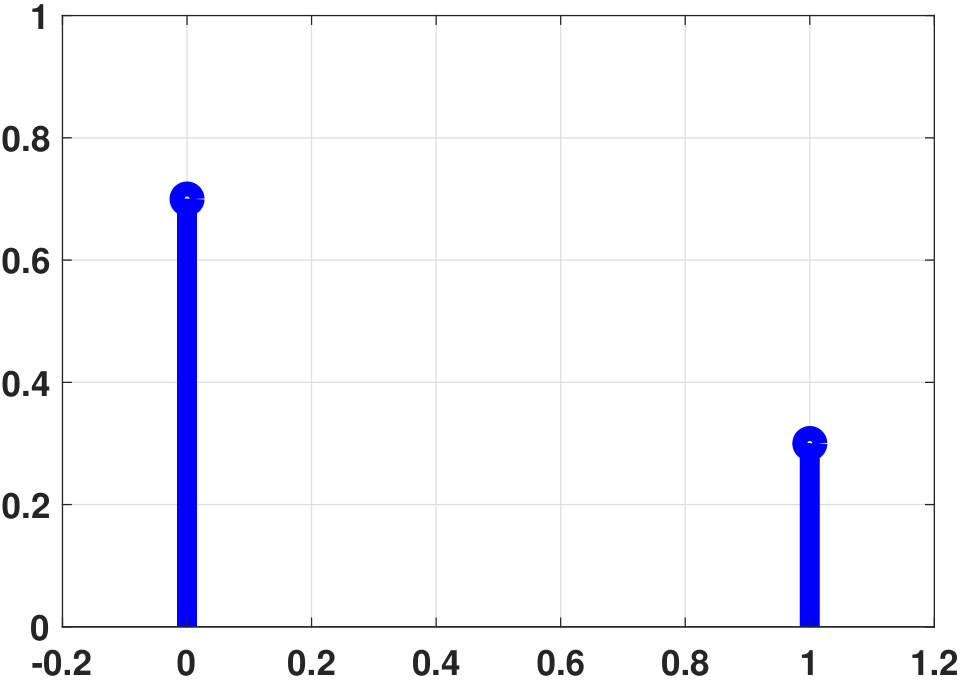
print(mean, var)In both MATLAB and Python, we can plot the PMF of a Bernoulli random variable, such as the one shown in Figure 3.22. To do this in MATLAB, we call the function binopdf, with the evaluation points specified by x.
% MATLAB code to plot the PMF of a Bernoulli
    p = 0.3;
    x = [0,1];
    f = binopdf(x,1,p);
    stem(x, f, `bo', `LineWidth', 8);
In Python, we construct a random variable rv. With rv, we can call its PMF rv.pmf:
# Python code to plot the PMF of a Bernoulli
    import numpy as np
    import matplotlib.pyplot as plt
    import scipy.stats as stats
    p = 0.3
    rv = stats.bernoulli(p)
    x  = np.linspace(0, 1, 2)
    f  = rv.pmf(x)
    plt.plot(x, f, `bo', ms=10);
    plt.vlines(x, 0, f, colors=`b', lw=5, alpha=0.5);
When will a Bernoulli random variable have the maximum variance?
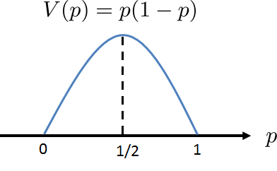
Let us take a look at the variance of the Bernoulli random variable. For any given \(p\), the variance is \(p(1-p)\). This is a quadratic equation. If we let \(V(p) = p(1-p)\), we can show that the maximum is attained at \(p = 1/2\). To see this, take the derivative of \(V(p)\) with respect to \(p\). This will give us \(\frac{d}{dp}V(p) = 1-2p\). Equating to zero yields \(1-2p = 0\), so \(p = 1/2\). We know that \(p = 1/2\) is a maximum and not a minimum point because the second-order derivative \(V''(p) = -2\), which is negative. Therefore \(V(p)\) is maximized at \(p = 1/2\). Now, since \(0 \le p \le 1\), we also know that \(V(0) = 0\) and \(V(1) = 0\). Therefore, the variance is minimized at \(p = 0\) and \(p = 1\). Figure 3.23 shows a graph of the variance.
Does this result make sense? Why is the variance maximized at \(p = 1/2\)? If we think about this problem more carefully, we realize that a Bernoulli random variable represents a coin-flip experiment. If the coin is biased such that it always gives heads, on the one hand, it is certainly a bad coin. However, on the other hand, the variance is zero because there is nothing to vary; you will certainly get heads. The same situation happens if the coin is biased towards tails. However, if the coin is fair, i.e., \(p = 1/2\), then the variance is large because we only have a 50% chance of getting a head or a tail whenever we flip a coin. Nothing is certain in this case. Therefore, the maximum variance happening at \(p = 1/2\) matches our intuition.
Rademacher random variable
A slight variation of the Bernoulli random variable is the Rademacher random variable, which has two states: \(+1\) and \(-1\). The probability of getting \(+1\) or \(-1\) is each \(1/2\). Therefore, the PMF of a Rademacher random variable is
Show that if \(X\) is a Rademacher random variable then \((X+1)/2 \sim \text{Bernoulli}(1/2)\). Also show the converse: If \(Y \sim \text{Bernoulli}(1/2)\) then \(2Y-1\) is a Rademacher random variable.
Since \(X\) can either be \(+1\) or \(-1\), we show that if \(X = +1\) then \((X+1)/2 = 1\) and if \(X = -1\) then \((X+1)/2 = 0\). The probabilities of getting \(+1\) and \(-1\) are equal. Thus, the probabilities of getting \((X+1)/2 = 1\) and \(0\) are also equal. So the resulting random variable is Bernoulli(1/2). The other direction can be proved similarly.
Bernoulli in social networks: the Erdos-R\'enyi graph
The study of networks is a big branch of modern data science. It includes social networks, computer networks, traffic networks, etc. The history of network science is very long, but one of the most basic models of a network is the Erdos-R\'enyi graph, named after Paul Erdos and Alfr\'ed R\'enyi. The underlying probabilistic model of the Erdos-R\'enyi graph is the Bernoulli random variable.
To see how a graph can be constructed from a Bernoulli random variable, we first introduce the concept of a graph. A graph contains two elements: nodes and edges. For node \(i\) and node \(j\), we denote the edge connecting \(i\) and \(j\) as \(A_{ij}\). Therefore, if we have \(N\) nodes, then we can construct a matrix \(\mA\) of size \(N \times N\). We call this matrix the adjacency matrix. For example, the adjacency matrix
will have edges for node pairs \((1,2)\), \((1,3)\), and \((3,4)\). Note that in this example we assume that the adjacency matrix is symmetric, meaning that the graph is undirected. The “1” in the adjacency matrix indicates there is an edge, and “0” indicates there is no edge. So \(\mA\) represents a binary graph.
The Erdos-R\'enyi graph model says that the probability of getting an edge is an independent Bernoulli random variable. That is
for \(i < j\). If we model the graph in this way, then the parameter \(p\) will control the density of the graph. High values of \(p\) mean that there is a higher chance for an edge to be present.
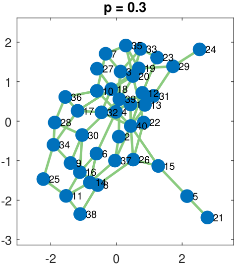
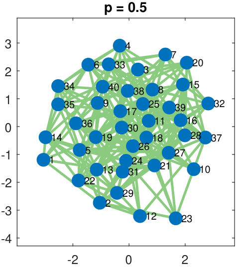
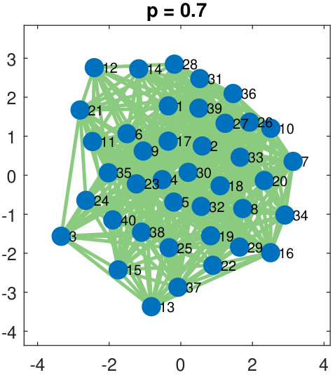
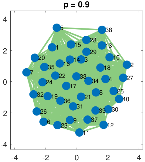
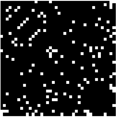
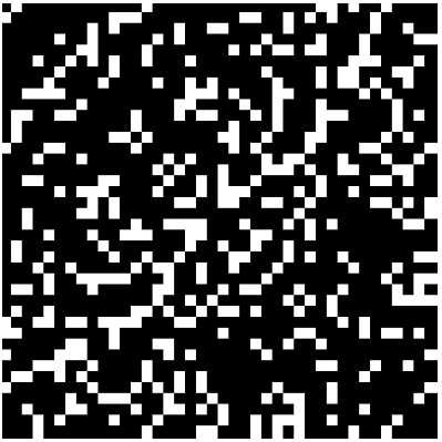
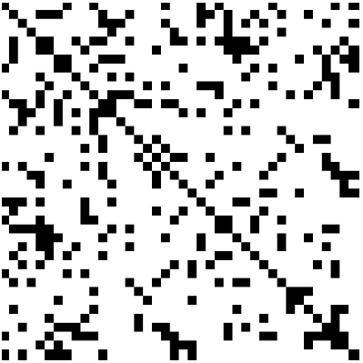
To illustrate the idea of an Erdos-R\'enyi graph, we show in Figure 3.24 a graph of 40 nodes. The edges are randomly selected by flipping a Bernoulli random variable with parameter \(p = 0.3, 0.5, 0.7, 0.9\). As we can see in the figure, a small value of \(p\) gives a graph with very sparse connectivity, whereas a large value of \(p\) gives a very densely connected graph. The bottom row of Figure 3.24 shows the corresponding adjacency matrices. Here, a white pixel denotes “1” in the matrix and a black pixel denotes “0” in the matrix.

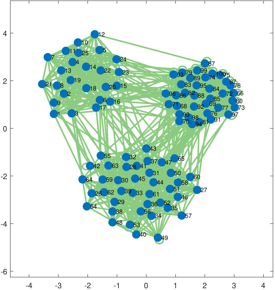
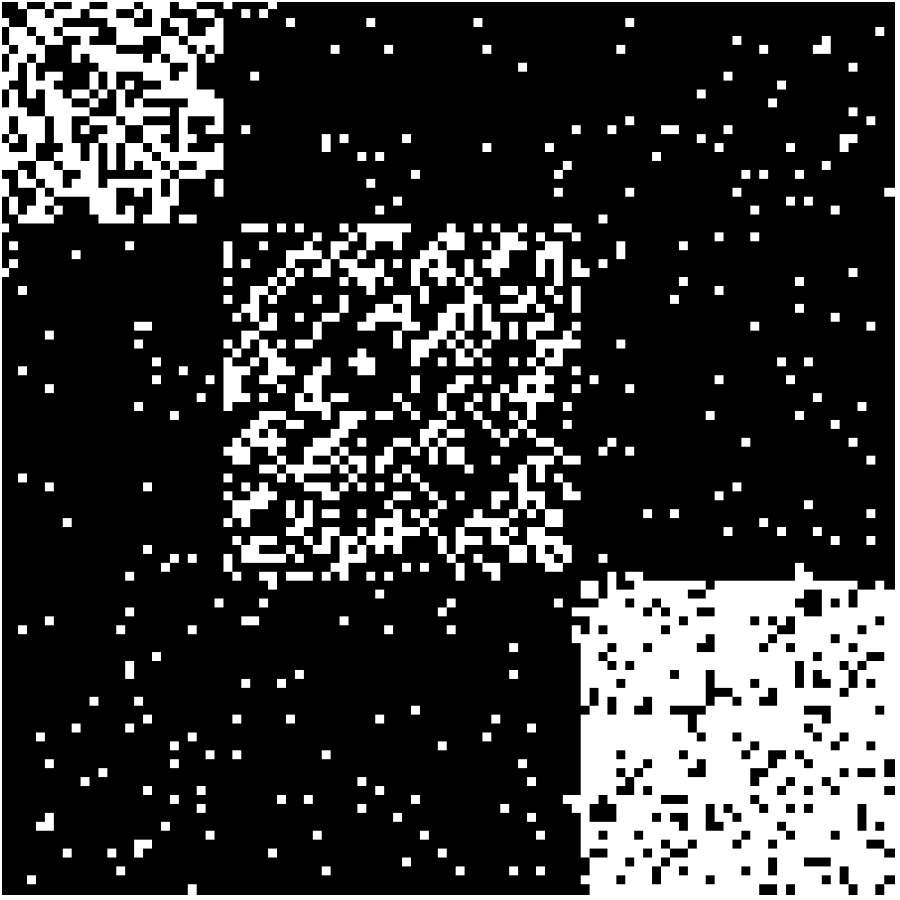
While Erdos-R\'enyi graphs are elementary, their variations can be realistic models of social networks. The stochastic block model is one such model. In a stochastic block model, nodes form small communities within a large network. For example, there are many majors in a university. Students within the same major tend to have more interactions than with students of another major. The stochastic block model achieves this goal by partitioning the nodes into communities. Within each community, the nodes can have a high degree of connectivity. Across different communities, the connectivity will be much lower. Figure 3.25 illustrates a network and the corresponding adjacency matrix. In this example, the network has three communities.
In network analysis, one of the biggest problems is determining the community structure and recovering the underlying probabilities. The former task is about grouping the nodes into blocks. This is a nontrivial problem because in practice the nodes are never arranged nicely, as shown in Figure 3.25. For example, why should Alice be node 1 and Bob be node 2? Since we never know the correct ordering of the nodes, partitioning the nodes into blocks requires various estimation techniques such as clustering or iterative estimation. Recovering the underlying probability is also not easy. Given an adjacency matrix, why can we assume that the underlying network is a stochastic block model? Even if the model is correct, there will be imperfect grouping in the previous step. As such, estimating the underlying probability in the presence of these uncertainties would pose additional challenges.
Today, network analysis remains one of the hottest areas in data science. Its importance derives from its broad scope and impact. It can be used to analyze social networks, opinion polls, marketing, or even genome analysis. Nevertheless, the starting point of these advanced subjects is the Bernoulli random variable, the random variable of a coin flip!
3.5.2Binomial random variable
Suppose we flip the coin \(n\) times and count the number of heads. Since each coin flip is a random variable (Bernoulli), the sum is also a random variable. It turns out that this new random variable is the binomial random variable.
Let \(X\) be a binomial random variable. Then, the PMF of \(X\) is
where \(0 < p < 1\) is the binomial parameter, and \(n\) is the number of trials. We write $$X \sim \mathrm{Binomial}(n,p)$$ to say that \(X\) is drawn from a binomial distribution with a parameter \(p\) of size \(n\).
To understand the meaning of a binomial random variable, consider a simple experiment consisting of flipping a coin three times. We know that all possible cases are HHH, HHT, HTH, THH, TTH, THT, HTT and TTT. Now, suppose we define \(X\) = number of heads. We want to write down the probability mass function. Effectively, we ask: What is the probability of getting 0 head, one head, two heads, and three heads? We can, of course, count and get the answer right away for a fair coin. However, suppose the coin is unfair, i.e., the probability of getting a head is \(p\) whereas that of a tail is \(1-p\). The probability of getting each of the 8 cases is shown in Figure 3.26 below.
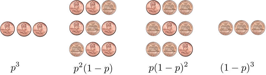
Here are the detailed calculations. Let us start with \(X = 3\).
where \((a)\) holds because the three events are independent. (Recall that if \(A\) and \(B\) are independent then \(\Pb[A \cap B] = \Pb[A]\Pb[B]\).) \((b)\) holds because each \(\Pb[\{\text{H}\}] = p\) by definition. With exactly the same argument, we can show that \(p_X(0) = \Pb[\{\text{TTT}\}] = (1-p)^3\).
Now, let us look at \(p_X(2)\), i.e., 2 heads. This probability can be calculated as follows:
where \((c)\) holds because the three events HHT, HTH and THH are disjoint in the sample space. Note that we are not using the independence argument in \((c)\) but the disjoint argument. We should not confuse the two. The step in \((d)\) uses independence, because each coin flip is independent.
The above calculation shows an interesting phenomenon: Although the three events HHT, HTH, and THH are different (in fact, disjoint), the number of heads in all the cases is the same. This happens because when counting the number of heads, the ordering of the heads and tails does not matter. So the same problem can be formulated as finding the number of combinations of \(\{\) 2 heads and 1 tail \(\}\), which in our case is \({3 \choose 2} = 3\).
To complete the story, let us also try \(p_X(1)\). This probability is
Again, we see that the combination \({3 \choose 1} = 3\) appears in front of the \(p(1-p)^2\).
In general, the way to interpret the binomial random variable is to decouple the probabilities \(p\), \((1-p)\), and the number of combinations \({n \choose k}\):
The running index \(k\) should go with \(0, 1, \ldots, n\). It starts with 0 because there could be zero heads in the sample space. Furthermore, we note that in this definition, two parameters are driving a binomial random variable: the number of Bernoulli trials \(n\) and the underlying probability for each coin flip \(p\). As such, the notation for a binomial random variable is \(\text{Binomial}(n,p)\), with two arguments.
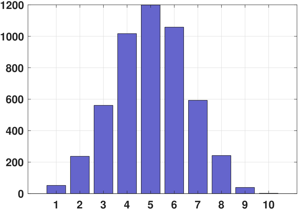
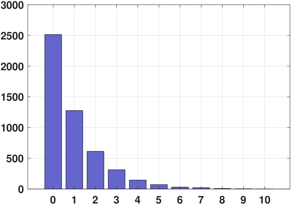
The histogram of a binomial random variable is shown in Figure 3.27(a). Here, we consider the example where \(n = 10\) and \(p = 0.5\). To generate the histogram, we use 5000 samples. In MATLAB and Python, generating binomial random variables as in Figure 3.27(a) can be done by calling binornd and np.random.binomial.
% MATLAB code to generate 5000 Binomial random variables
    p = 0.5;
    n = 10;
    X = binornd(n,p,[5000,1]);
    [num, ~] = hist(X, 10);
bar( num,`FaceColor',[0.4, 0.4, 0.8]);# Python code to generate 5000 Binomial random variables
import numpy as np
import matplotlib.pyplot as plt
p = 0.5
n = 10
X = np.random.binomial(n,p,size=5000)
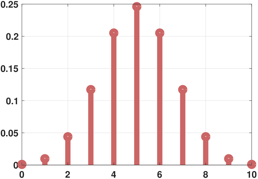
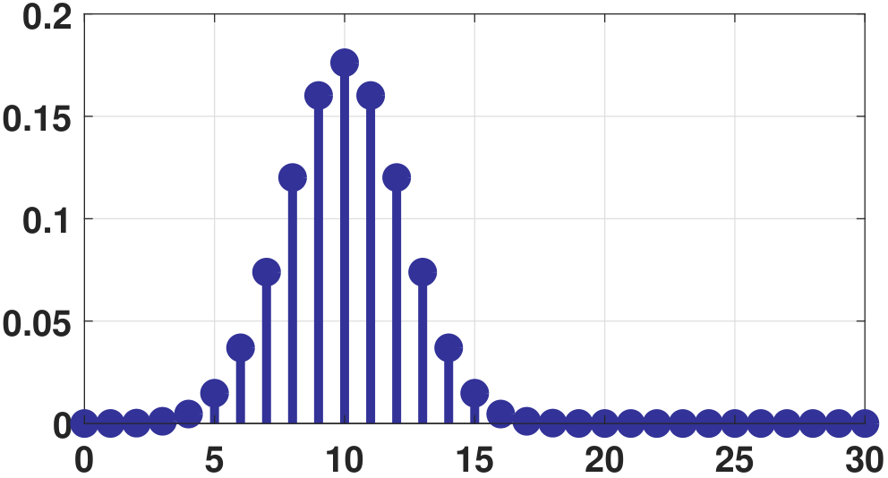
plt.hist(X,bins=`auto');Generating the ideal PMF of a binomial random variable as shown in Figure 3.27(b) can be done by calling binopdf in MATLAB. In Python, we can define a random variable rv through stats.binom, and call the PMF using rv.pmf.
% MATLAB code to generate a binomial PMF
    p = 0.5;
    n = 10;
    x = 0:10;
    f = binopdf(x,n,p);
stem(x, f, 'o', 'LineWidth', 8, 'Color', [0.8, 0.4, 0.4]);# Python code to generate a binomial PMF
import numpy as np
import matplotlib.pyplot as plt
import scipy.stats as stats
p = 0.5
n = 10
rv = stats.binom(n,p)
x = np.arange(11)
f = rv.pmf(x)
plt.plot(x, f, 'bo', ms=10);
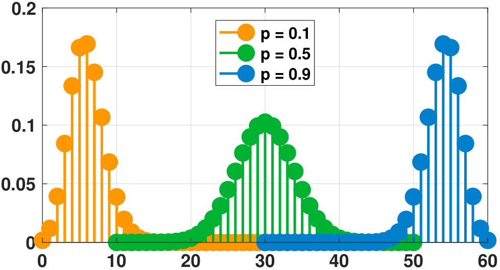
plt.vlines(x, 0, f, colors='b', lw=5, alpha=0.5);The shape of the binomial PMF is shown in Figure 3.28. In this set of figures, we vary one of the two parameters \(n\) and \(p\) while keeping the other fixed. In Figure 3.28(a), we fix \(n = 60\) and plot three sets of \(p = 0.1, 0.5, 0.9\). For small \(p\) the PMF is skewed towards the left, and for large \(p\) the PMF is skewed toward the right. Figure 3.28(b) shows the PMF for a fixed \(p = 0.5\). As we increase \(n\), the centroid of the PMF moves towards the right. Thus we should expect the mean of a binomial random variable to increase with \(n\). Another interesting observation is that as \(n\) increases, the shape of the PMF approaches the Gaussian function (the bell-shaped curve). We will explain the reason for this when we discuss the Central Limit Theorem.
The expectation, second moment, and variance of a binomial random variable are summarized in Theorem def: moment properties of binomial.
If \(X \sim \mathrm{Binomial}(n,p)\), then
We will prove that \(\E[X] = np\) from first principles. For \(\E[X^2]\) and \(\Var[X]\), we will skip the proofs here and will introduce a “shortcut” later.
Proof. Let us start with the definition.
Note that we have shifted the index from \(k = 0\) to \(k=1\). Now let us apply a trick:
Using this trick, we can show that
With a simple substitution of \(\ell = k-1\), the above equation can be rewritten as
In MATLAB, the mean and variance of a binomial random variable can be found by calling the command binostat(n,p) (MATLAB).
In Python, the command is rv = stats.binom(n,p) followed by calling rv.stats.
% MATLAB code to compute the mean and var of a binomial rv
    p = 0.5;
    n = 10;
[M,V] = binostat(n, p)# Python code to compute the mean and var of a binomial rv
import scipy.stats as stats
p = 0.5
n = 10
rv = stats.binom(n,p)
M, V = rv.stats(moments=`mv')
print(M, V)An alternative view of the binomial random variable. As we discussed, the origin of a binomial random variable is the sum of a sequence of Bernoulli random variables. Because of this intrinsic definition, we can derive some useful results by exploiting this fact. To do so, let us define \(I_1,\ldots,I_n\) as a sequence of Bernoulli random variables with \(I_j \sim \mathrm{Bernoulli}(p)\) for all \(j = 1,\ldots,n\). Then the resulting variable
is a binomial random variable of size \(n\) and parameter \(p\). Using this definition, we can compute the expectation as follows:
In this derivation, the step \((a)\) depends on a useful fact about expectation (which we have not yet proved): For any two random variables \(X\) and \(Y\), it holds that \(\E[X+Y] = \E[X] + \E[Y]\). Therefore, we can show that the expectation of \(X\) is \(np\). This line of argument not only simplifies the proof but also provides a good intuition of the expectation. If each coin flip has an expectation of \(\E[I_i] = p\), then the expectation of the sum should be simply \(n\) times \(p\), giving \(np\).
How about the variance? Again, we are going to use a very useful fact about variance: If two random variables \(X\) and \(Y\) are independent, then \(\Var[X+Y] = \Var[X] + \Var[Y]\). With this result, we can show that
Finally, using the fact that \(\Var[X] = \E[X^2] - \mu^2\), we can show that
Show that the binomial PMF sums to 1.
We use the binomial theorem to prove this result:
The CDF of the binomial random variable is not very informative. It is basically the cumulative sum of the PMF:
The shapes of the PMF and the CDF is shown in Figure 3.29.
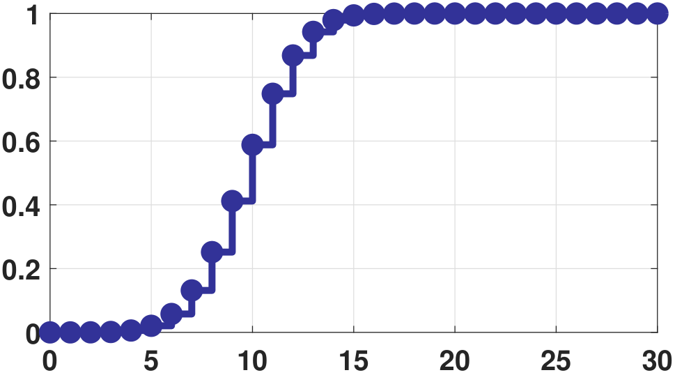
In MATLAB, plotting the CDF of a binomial can be done by calling the function binocdf. You may also call f = binopdf(x,n,p), and define F = cumsum(f) as the cumulative sum of the PMF. In Python, the corresponding command is rv = stats.binom(n,p) followed by rv.cdf.
% MATLAB code to compute the mean and var of a binomial rv
    x = 0:10;
    p = 0.5;
    n = 10;
    F = binocdf(x,n,p);
figure; stairs(x,F,`.-',`LineWidth',4,`MarkerSize',30);# Python code to compute the mean and var of a binomial rv
import numpy as np
import matplotlib.pyplot as plt
import scipy.stats as stats
p = 0.5
n = 10
rv = stats.binom(n,p)
x = np.arange(11)
F = rv.cdf(x)
plt.plot(x, F, 'bo', ms=10);
plt.vlines(x, 0, F, colors='b', lw=5, alpha=0.5);3.5.3Geometric random variable
In some applications, we are interested in trying a binary experiment until we succeed. For example, we may want to keep calling someone until the person picks up the call. In this case, the random variable can be defined as the outcome of many failures followed by a final success. This is called the geometric random variable.
Let \(X\) be a geometric random variable. Then, the PMF of \(X\) is
where \(0 < p < 1\) is the geometric parameter. We write $$X \sim \mathrm{Geometric}(p)$$ to say that \(X\) is drawn from a geometric distribution with a parameter \(p\).
A geometric random variable is easy to understand. We define it as Bernoulli trials with \(k-1\) consecutive failures followed by one success. This can be seen from the definition:
Note that in geometric random variables, there is no \({n \choose k}\) because we must have \(k-1\) consecutive failures before one success. There is no alternative combination of the sequence.
The histogram and PMF of a geometric random variable are illustrated in Figure 3.30. Here, we assume that \(p = 0.5\).
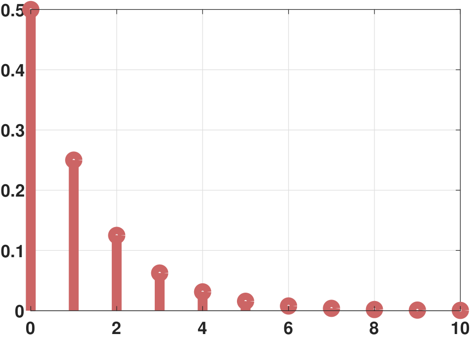
In MATLAB, generating geometric random variables can be done by calling the commands geornd. In Python, it is np.random.geometric.
% MATLAB code to generate 1000 geometric random variables
    p = 0.5;
    X = geornd(p,[5000,1]);
    [num, ~] = hist(X, 0:10);
bar(0:10, num, `FaceColor',[0.4, 0.4, 0.8]);# Python code to generate 1000 geometric random variables
import numpy as np
import matplotlib.pyplot as plt
p = 0.5
X = np.random.geometric(p,size=1000)
plt.hist(X,bins=`auto');To generate the PMF plots, we use geopdf and rv = stats.geom.
% MATLAB code to generate geometric PMF
    p = 0.5; x = 0:10;
    f = geopdf(x,p);
stem(x, f, `o', `LineWidth', 8, `Color', [0.8, 0.4, 0.4]);# Python code to generate 1000 geometric random variables
import numpy as np
import matplotlib.pyplot as plt
import scipy.stats as stats
x = np.arange(1,11)
rv = stats.geom(p)
f = rv.pmf(x)
plt.plot(x, f, `bo', ms=8, label=`geom pmf')
plt.vlines(x, 0, f, colors=`b', lw=5, alpha=0.5)Show that the geometric PMF sums to one.
We can apply infinite series to show the result:
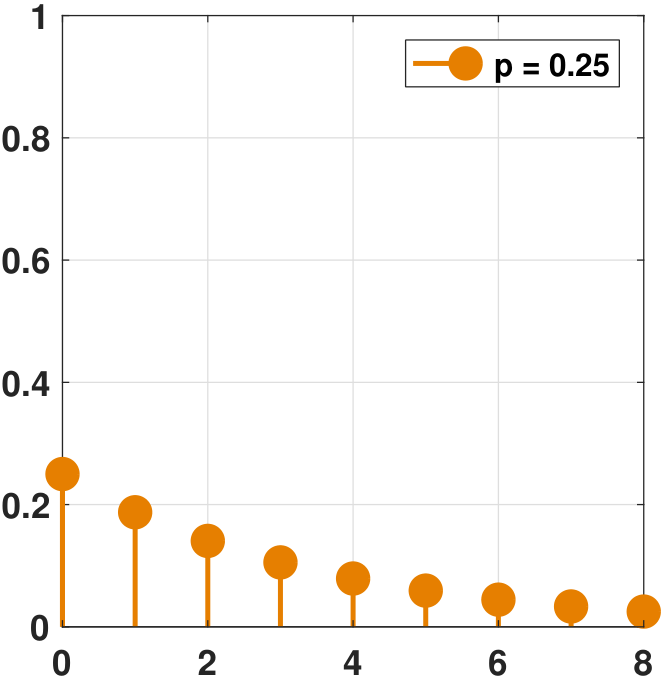
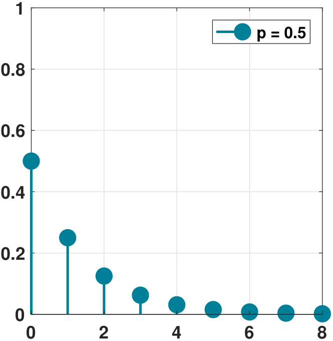
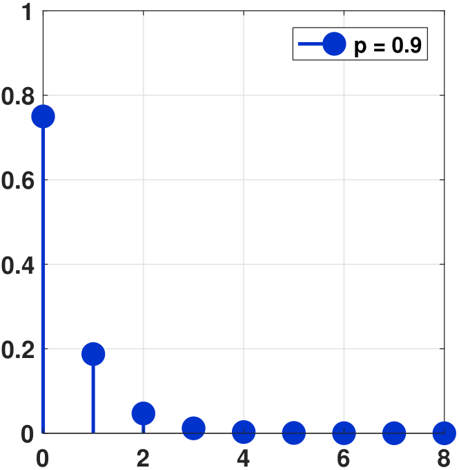
It is interesting to compare the shape of the PMFs for various values of \(p\). In Figure 3.31 we show the PMFs. We vary the parameter \(p = 0.25, 0.5, 0.9\). For small \(p\), the PMF starts with a low value and decays at a slow speed. The opposite happens for a large \(p\), where the PMF starts with a high value and decays rapidly.
Furthermore, we can derive the following properties of the geometric random variable.
If \(X \sim \mathrm{Geometric}(p)\), then
Proof. We will prove that the mean is \(1/p\) and leave the second moment and variance as an exercise.
where \((a)\) follows from the infinite series identity in Chapter 1.
■3.5.4Poisson random variable
In many physical systems, the arrivals of events are typically modeled as a Poisson random variable, e.g., photon arrivals, electron emissions, and telephone call arrivals. In social networks, the number of conversations per user can also be modeled as a Poisson. In e-commerce, the number of transactions per paying user is again modeled using a Poisson.
Let \(X\) be a Poisson random variable. Then, the PMF of \(X\) is
where \(\lambda > 0\) is the Poisson rate. We write $$X \sim \mathrm{Poisson}(\lambda)$$ to say that \(X\) is drawn from a Poisson distribution with a parameter \(\lambda\).
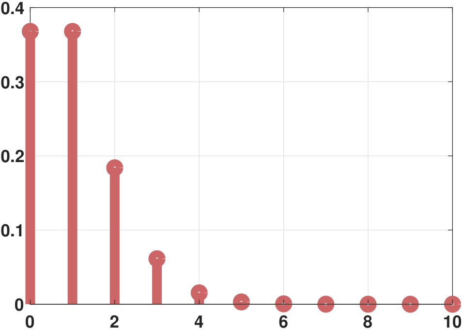
In this definition, the parameter \(\lambda\) determines the rate of the arrival. The histogram and PMF of a Poisson random variable are illustrated in Figure 3.32. Here, we assume that \(\lambda = 1\).
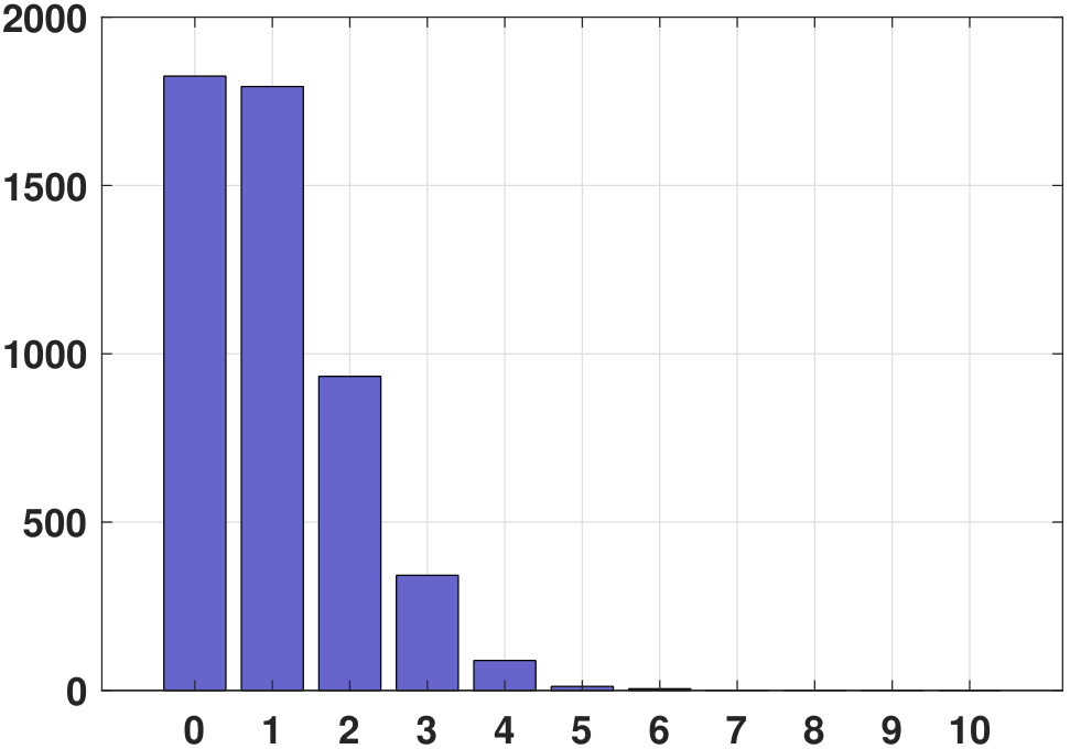
The MATLAB code and Python code used to generate the histogram are shown below.
% MATLAB code to generate 5000 Poisson numbers
    lambda = 1;
    X = poissrnd(lambda,[5000,1]);
    [num, ~] = hist(X, 0:10);
bar(0:10, num, `FaceColor',[0.4, 0.4, 0.8]);# Python code to generate 5000 Poisson random variables
import numpy as np
import matplotlib.pyplot as plt
lambd = 1
X = np.random.poisson(lambd,size=5000)
plt.hist(X,bins=`auto');For the PMF, in MATLAB we can call poisspdf, and in Python we can call rv.pmf with rv = stats.poisson.
% MATLAB code to plot the Poisson PMF
    lambda = 1;
    x = 0:10;
    f = poisspdf(x,lambda);
stem(x, f, `o', `LineWidth', 8, `Color', [0.8, 0.4, 0.4]);# Python code to plot the Poisson PMF
import numpy as np
import matplotlib.pyplot as plt
import scipy.stats as stats
x = np.arange(0,11)
rv = stats.poisson(lambd)
f = rv.pmf(x)
plt.plot(x, f, `bo', ms=8, label=`geom pmf')
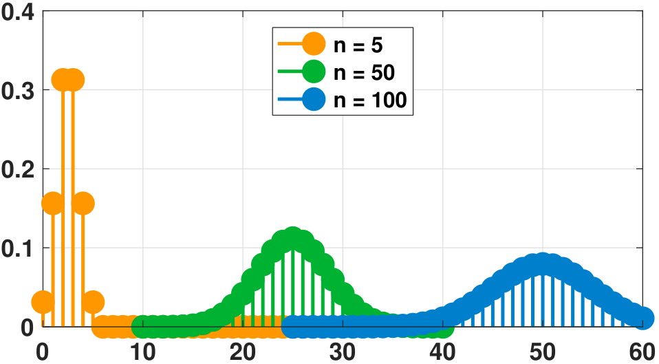
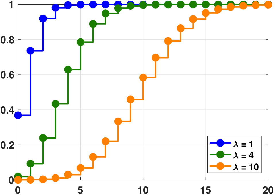
plt.vlines(x, 0, f, colors=`b', lw=5, alpha=0.5)The shape of the Poisson PMF changes with \(\lambda\). As illustrated in Figure 3.33, \(p_X(k)\) is more concentrated at lower values for smaller \(\lambda\) and becomes spread out for larger \(\lambda\). Thus, we should expect that the mean and variance of a Poisson random variable will change together as a function of \(\lambda\). In the same figure, we show the CDF of a Poisson random variable. The CDF of a Poisson is

Let \(X\) be a Poisson random variable with parameter \(\lambda\). Find \(\Pb[X > 4]\) and \(\Pb[X \le 5]\).
Show that the Poisson PMF sums to 1.
We use the exponential series to prove this result:
Poisson random variables in practice
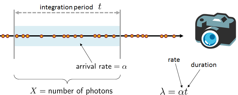
(1) Computational photography. In computational photography, the Poisson random variable is one of the most widely used models for photon arrivals. The reason pertains to the origin of the Poisson random variable, which we will discuss shortly. When photons are emitted from the source, they travel through the medium as a sequence of independent events. During the integration period of the camera, the photons are accumulated to generate a voltage that is then translated to digital bits.
If we assume that the photon arrival rate is \(\alpha\) (photons per second), and suppose that the total amount of integration time is \(t\), then the average number of photons that the sensor can see is \(\alpha t\). Let \(X\) be the number of photons seen during the integration time. Then if we follow the Poisson model, we can write down the PMF of \(X\):
Therefore, if a pixel is bright, meaning that \(\alpha\) is large, then \(X\) will have a higher likelihood of landing on a large number.
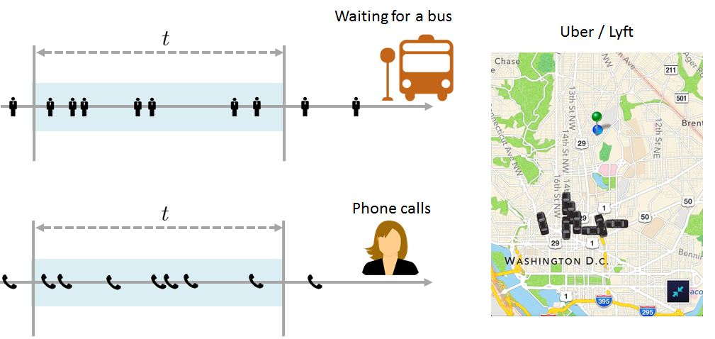
(2) Traffic model. The Poisson random variable can be used in many other problems. For example, we can use it to model the number of passengers on a bus or the number of spam phone calls. The required modification to Figure 3.34 is almost trivial: merely replace the photons with your favorite cartoons, e.g., a person or a phone, as shown in Figure 3.35. In the United States, shared-ride services such as Uber and Lyft need to model the vacant cars and the passengers. As long as they have an arrival rate and certain degrees of independence between events, the Poisson random variable will be a good model.
As you can see from these examples, the Poisson random variable has broad applicability. Before we continue our discussion of its applications, let us introduce a few concepts related to the Poisson random variable.
Properties of a Poisson random variable
We now derive the mean and variance of a Poisson random variable.
If \(X \sim \mathrm{Poisson}(\lambda)\), then
Proof. Let us first prove the mean. It can be shown that
The second moment can be computed as
The variance can be computed using \(\Var[X] = \E[X^2] - \mu^2\).
■To compute the mean and variance of a Poisson random variable, we can call poisstat in MATLAB and rv.stats(moments=`mv') in Python.
% MATLAB code to compute Poisson statistics
    lambda = 1;
[M,V] = poisstat(lambda);# Python code to compute Poisson statistics
import scipy.stats as stats
lambd = 1
rv = stats.poisson(lambd)
M, V = rv.stats(moments='mv')The Poisson random variable is special in the sense that the mean and the variance are equal. That is, if the mean arrival number is higher, the variance is also higher. This is very different from some other random variables, e.g., the normal random variable where the mean and variance are independent. For certain engineering applications such as photography, this plays an important role in defining the signal-to-noise ratio. We will come back to this point later.
Origin of the Poisson random variable
We now address one of the most important questions about the Poisson random variable: Where does it come from? Answering this question is useful because the derivation process will reveal the underlying assumptions that lead to the Poisson PMF. When you change the problem setting, you will know when the Poisson PMF will hold and when the Poisson PMF will fail.
Our approach to addressing this problem is to consider the photon arrival process. (As we have shown, there is conceptually no difference if you replace the photons with pedestrians, passengers, or phone calls.) Our derivation follows the argument of J. Goodman, Statistical Optics, Section 3.7.2.
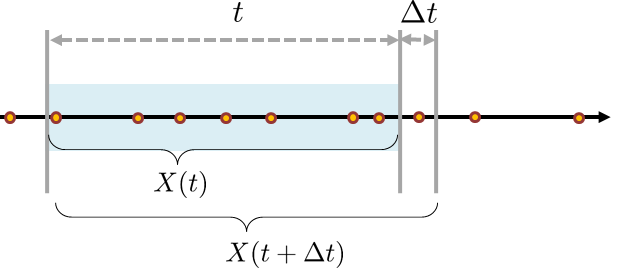
To begin with, we consider a photon arrival process. The total number of photons observed over an integration time \(t\) is defined as \(X(t)\). Because \(X(t)\) is a Poisson random variable, its arguments must be integers. The probability of observing \(X(t) = k\) is therefore \(\Pb[X(t) = k]\). Figure 3.36 illustrates the notations and concepts.
We propose three hypotheses with the photon arrival process:
For sufficiently small \(\Delta t\), the probability of a small impulse occurring in the time interval \([t, t+\Delta t]\) is equal to the product of \(\Delta t\) and the rate \(\lambda\), i.e., $$\Pb[X(t+\Delta t) - X(t) = 1] = \lambda \Delta t.$$ This is a linearity assumption, which typically holds for a short duration of time.
- For sufficiently small \(\Delta t\), the probability that more than one impulse falls in \(\Delta t\) is negligible. Thus, we have that \(\Pb[X(t+\Delta t) - X(t) = 0] = 1-\lambda \Delta t\).
- The number of impulses in non-overlapping time intervals is independent.
The significance of these three hypotheses is that if the underlying photon arrival process violates any of these assumptions, then the Poisson PMF will not hold. One example is the presence of scattering effects, where a photon has a certain probability of going off due to the scattering medium and a certain probability of coming back. In this case, the events will no longer be independent.
Assuming that these hypotheses hold, then at time \(t+\Delta t\), the probability of observing \(X(t+\Delta t) = k\) can be computed as
By rearranging the terms we show that
Setting the limit of \(\Delta t \rightarrow 0\), we arrive at an ordinary differential equation
We claim that the Poisson PMF, i.e.,
would solve this differential equation. To see this, we substitute the PMF into the equation. The left-hand side gives us
which is the right-hand side of the equation. To retrieve the basic form of Poisson, we can just set \(t = 1\) in the PMF so that
- sep0em
- We assume independent arrivals.
- Probability of seeing one event is linear with the arrival rate.
- Time interval is short enough so that you see either one event or no event.
- Poisson is derived by solving a differential equation based on these assumptions.
- Poisson becomes invalid when these assumptions are violated, e.g., in the case of scattering of photons due to turbid medium.
There is an alternative approach to deriving the Poisson PMF. The idea is to drive the parameter \(n\) in the binomial random variable to infinity while pushing \(p\) to zero. In this limit, the binomial PMF will converge to the Poisson PMF. We will discuss this shortly. However, we recommend the physics approach we have just described because it has a rich meaning and allows us to validate our assumptions.
Poisson approximation to binomial
We present one additional result about the Poisson random variable. The result shows that Poisson can be regarded as a limiting distribution of a binomial random variable.
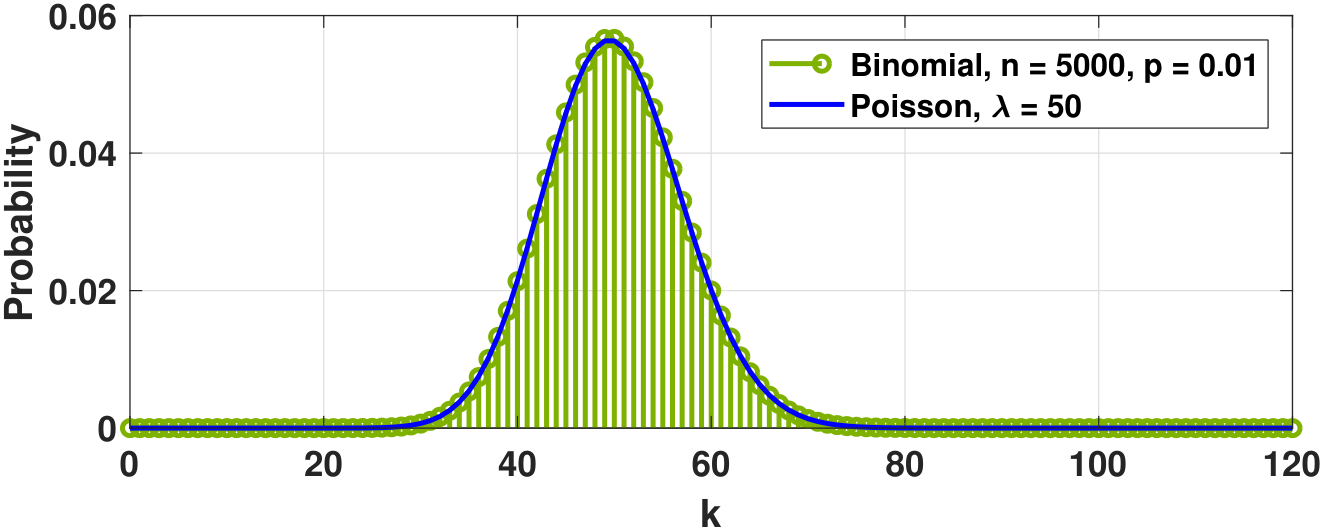
(Poisson approximation to binomial). For small \(p\) and large \(n\),
where \(\lambda \bydef np\).
Before we prove the result, let us see how close the approximation can be. In Figure 3.37, we show a binomial distribution and a Poisson approximation. The closeness of the approximation can easily be seen.
In MATLAB, the code to approximate a binomial distribution with a Poisson formula is shown below. Here, we draw 10,000 random binomial numbers and plot their histogram. On top of the plot, we use poisspdf to compute the Poisson PMF. This gives us Figure 3.37. A similar set of commands can be called in Python.
% MATLAB code to approximate binomial using Poisson
    n = 1000; p = 0.05;
    X = binornd(n,p,[10000,1]);
    t = 0:100;
    [num,val] = hist(X,t);
    lambda = n*p;
    f_pois = poisspdf(t,lambda);
    bar(num/10000,`FaceColor',[0.9 0.9 0],`BarWidth',1); hold on;
plot(f_pois, `LineWidth', 4);# Python code to approximate binomial using Poisson
import numpy as np
import matplotlib.pyplot as plt
import scipy.stats as stats
n = 1000; p = 0.05
rv1 = stats.binom(n,p)
X = rv1.rvs(size=10000)
plt.figure(1); plt.hist(X,bins=np.arange(0,100));
rv2 = stats.poisson(n*p)
f = rv2.pmf(bin)
plt.figure(2); plt.plot(f);Proof. Let \(\lambda = np\). Then,
We claim that \(\left(1-\frac{\lambda}{n}\right)^{n} \rightarrow e^{-\lambda}\). This can be proved by noting that
It then follows that \(\log \left(1-\frac{\lambda}{n}\right) \approx -\frac{\lambda}{n}\). Hence, \(\left(1-\frac{\lambda}{n}\right)^{n} \approx e^{-\lambda}\)
■Consider an optical communication system. The bit arrival rate is \(10^{9}\) bits/sec, and the probability of having one error bit is \(10^{-9}\). Suppose we want to find the probability of having five error bits in one second.
Let \(X\) be the number of error bits. In one second there are \(10^9\) bits. Since we do not know the location of these 5 bits, we have to enumerate all possibilities. This leads to a binomial distribution. Using the binomial distribution, we know that the probability of having \(k\) error bits is
This quantity is difficult to calculate in floating-point arithmetic.
Using the Poisson approximation to the binomial, we can see that the probability can be approximated by
where \(\lambda = np = 10^9 (10^{-9})= 1\). Setting \(k=5\) yields \(\Pb[X=5] \approx 0.003\).
Photon arrival statistics
Poisson random variables are useful in computer vision, but you may skip this discussion if it is your first reading of the book.
The strong connection between Poisson statistics and physics makes the Poisson random variable a very good fit for many physical experiments. Here we demonstrate an application in modeling photon shot noise.
An image sensor is a photon-sensitive device which is used to detect incoming photons. In the simplest setting, we can model a pixel in the object plane as \(X_{m,n}\), for some 2D coordinate \([m,n] \in \R^2\). Written as an array, an \(M \times N\) image in the object plane can be visualized as
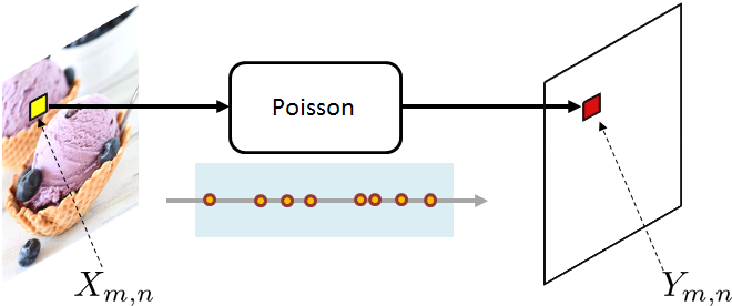
Without loss of generality, we assume that \(X_{m,n}\) is normalized so that \(0 \le X_{m,n} \le 1\) for every coordinate \([m,n]\). To model the brightness, we multiply \(X_{m,n}\) by a scalar \(\alpha > 0\). If a pixel \(\alpha X_{m,n}\) has a large value, then it is a bright pixel; conversely, if \(\alpha X_{m,n}\) has a small value, then it is a dark pixel. At a particular pixel location \([m,n] \in \R^2\), the observed pixel value \(Y_{m,n}\) is a random variable following the Poisson statistics. This situation is illustrated in Figure 3.38, where we see that an object-plane pixel will generate an observed pixel through the Poisson PMF. (The color of an image is often handled by a color filter array, which can be thought of as a wavelength selector that allows a specific wavelength to pass through.)
Written as an array, the image is
Here, by \(\text{Poisson}\{\alpha X_{m,n}\}\) we mean that \(Y_{m,n}\) is a random integer with probability mass
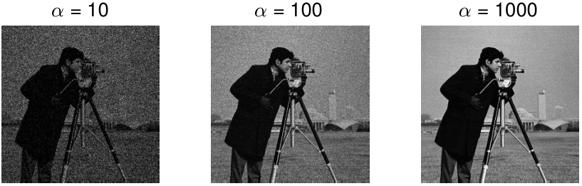
Note that this model implies that the images seen by our cameras are more or less an array of Poisson random variables. (We say “more or less” because of other sources of uncertainties such as read noise, dark current, etc.) Because the observed pixels \(Y_{m,n}\) are random variables, they fluctuate about the mean values, and hence they are noisy. We refer to this type of random fluctuation as the shot noise. The impact of the shot noise can be seen in Figure 3.39. Here, we vary the sensor gain level \(\alpha\). We see that for small \(\alpha\) the image is dark and has much random fluctuation. As \(\alpha\) increases, the image becomes brighter and the fluctuation becomes smaller.
In MATLAB, simulating the Poisson photon arrival process for an image requires the image-processing toolbox. The command to read an image is imread. Depending on the data type, the input array could be uint8 integers. To convert them to floating-point numbers between 0 and 1, we use the command im2double. Drawing Poisson measurements from the clean image is done using poissrnd. Finally, we can use imshow to display the image.
% MATLAB code to simulate a photon arrival process
    x0 = im2double(imread('cameraman.tif'));
    X  = poissrnd(10*x0);
    figure(1); imshow(x0, []);
    figure(2); imshow(X, []);
Similar commands can be found in Python with the help of the cv2 library. When reading an image, we call cv2.imread. The option 0 is used to read a gray-scale image; otherwise, we will have a 3-channel color image. The division /255 ensures that the input array ranges between 0 to 1. Generating the Poisson random numbers can be done using np.random.poisson, or by calling the statistics library with stats.poisson.rvs(10*x0). To display the images, we call plt.imshow, with the color map option set to cmap = 'gray'.
# Python code to simulate a photon arrival process
    import numpy as np
    import matplotlib.pyplot as plt
    import cv2
    x0 = cv2.imread('./cameraman.tif', 0)/255
    plt.figure(1); plt.imshow(x0,cmap='gray');
    X  = np.random.poisson(10*x0)
plt.figure(2); plt.imshow(X, cmap='gray');- sep0ex
- The Poisson random variable is used to model photon arrivals.
- Shot noise is the random fluctuation of the photon counts at the pixels. Shot noise is present even if you have an ideal sensor.
Signal-to-noise ratio of Poisson
Now let us answer a question we asked before. A Poisson random variable has a variance equal to the mean. Thus, if the scene is brighter, the variance will be larger. How come our simulation in Figure 3.39 shows that the fluctuation becomes smaller as the scene becomes brighter?
The answer to this question lies in the signal-to-noise ratio (SNR) of the Poisson random variable. The SNR of an image defines its quality. The higher the SNR, the better the image. The mathematical definition of SNR is the ratio between the signal power and the noise power. In our case, the SNR is
where \(Y = Y_{m,n}\) is one of the observed pixels and \(\lambda = \alpha X_{m,n}\) is the corresponding object pixel. In this equation, the step \((a)\) uses the properties of the Poisson random variable \(Y\) where \(\E[Y] = \Var[Y] = \lambda\). The result \(\text{SNR} = \sqrt{\lambda}\) is very informative. It says that if the underlying mean photon flux (which is \(\lambda\)) increases, the SNR increases at a rate of \(\sqrt{\lambda}\). So, yes, the variance becomes larger when the scene is brighter. However, the gain in signal \(\E[Y]\) overrides the gain in noise \(\sqrt{\Var[Y]}\). As a result, the big fluctuation in bright images is compensated by the strong signal. Thus, to minimize the shot noise one has to use a longer exposure to increase the mean photon flux. When the scene is dark and the aperture is small, shot noise is unavoidable.
Poisson modeling is useful for describing the problem. However, the actual engineering question is that, given a noisy observation \(Y_{m,n}\), how would you reconstruct the clean image \(X_{m,n}\)? This is a very difficult inverse problem. The typical strategy is to exploit the spatial correlations between nearby pixels, e.g., usually smooth except along some sharp edges. Other information about the image, e.g., the likelihood of obtaining texture patterns, can also be leveraged. Modern image-processing methods are rich, ranging from classical filtering techniques to deep neural networks. Static images are easier to recover because we can often leverage multiple measurements of the same scene to boost the SNR. Dynamic scenes are substantially harder when we need to track the motion of any underlying objects. There are also newer image sensors with better photon sensitivity. The problem of imaging in the dark is an important research topic in computational imaging. New solutions are developed at the intersection of optics, signal processing, and machine learning.
The end of our discussions on photon statistics.