eBook › Chapter 3 · Discrete Random Variables

Section 3.4

Expectation

When analyzing data, it is often useful to extract certain key parameters such as the mean and the standard deviation. The mean and the standard deviation can be seen from the lens of random variables. In this section, we will formalize the idea using expectation.

3.4.1Definition of expectation

Definition 3.4

The expectation of a random variable $X$ is

\E[X] = \sum_{x \in X(\Omega)}\, x \, p_X(x).

Expectation is the mean of the random variable $X$. Intuitively, we can think of $p_X(x)$ as the percentage of times that the random variable $X$ attains the value $x$. When this percentage is multiplied by $x$, we obtain the contribution of each $x$. Summing over all possible values of $x$ then yields the mean. To see this more clearly, we can write the definition as

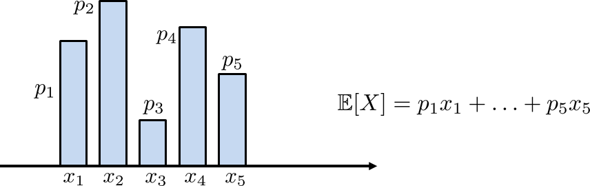
\E[X] = \underset{\text{\textcolor{blue}{sum over all states}}}{ \underbrace{ \qquad \qquad\sum_{x \in X(\Omega)}\qquad\qquad }} \qquad \underset{\text{\textcolor{blue}{a state $X$ takes}}}{\underbrace{\qquad x \qquad }} \quad \underset{\text{\textcolor{blue}{the percentage}}}{\underbrace{\qquad p_X(x) \qquad}}.

Figure 3.14 illustrates a PMF that contains five states $x_1,\ldots,x_5$. Corresponding to each state are $p_X(x_1), \ldots, p_X(x_5)$. For this PMF to make sense, we must assume that $p_X(x_1)+\cdots+p_X(x_5)=1$. To simplify notation, let us define $p_i \bydef p_X(x_i)$. Then the expectation of $X$ is just the sum of the products: value ($x_i$) times height ($p_i$). This gives $\E[X] = \sum_{i=1}^5 x_i p_X(x_i)$.

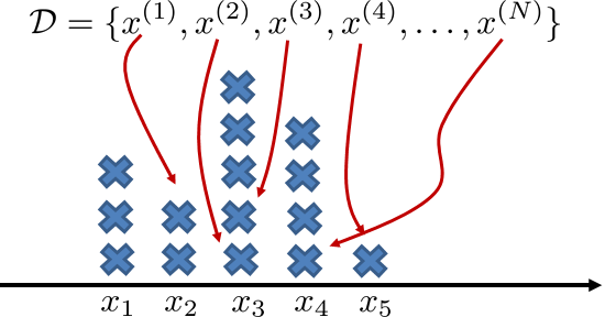
We emphasize that the definition of the expectation is exactly the same as the usual way we calculate the average of a dataset. When we calculate the average of a dataset $\calD = \{x^{(1)},x^{(2)},\ldots,x^{(N)}\}$, we sum up these $N$ samples and divide by the number of samples. This is what we called the empirical average or the sample average:

\text{average} = \frac{1}{N} \sum_{n=1}^N x^{(n)}.

Of course, in a typical dataset, these $N$ samples often take distinct values. But suppose that among these $N$ samples there are only $K$ different values. For example, if we throw a die a million times, every sample we record will be one of the six numbers. This situation is illustrated in Figure 3.15, where we put the samples into the correct bin storing these values. In this case, to calculate the average we are effectively doing a binning:

\text{average} = \frac{1}{N} \sum_{k=1}^K \text{value $x_k$} \;\; \times \;\; \text{number of samples with value $x_k$}.

Eq. (3.12) is exactly the same as Eq. (3.11), as long as the samples can be grouped into $K$ different values. With a little calculation, we can rewrite Eq. (3.12) as

\text{average} = \underset{\textcolor{blue}{\text{sum of all states}}}{\underbrace{\sum_{k=1}^K}} \underset{\textcolor{blue}{\text{a state $X$ takes}}}{\underbrace{\text{value $x_k$}}} \;\; \times \;\; \underset{\textcolor{blue}{\text{the percentage}}}{\underbrace{\frac{\text{number of samples with value $x_k$}}{N}}},

which is the same as the definition of expectation.

**Figure 3.15.** If we have a dataset $\calD$ containing $N$ samples, and if there are only $K$ distinct values, we can effectively put these $N$ samples into $K$ bins. Thus, the “average” (which is the sum divided by the number $N$) is exactly the same as our definition of expectation.

The difference between $\E[X]$ and the average is that $\E[X]$ is computed from the ideal histogram, whereas average is computed from the empirical histogram. When the number of samples $N$ approaches infinity, we expect the average to approximate $\E[X]$. However, when $N$ is small, the empirical average will have random fluctuations around $\E[X]$. Every time we experiment, the empirical average may be slightly different. Therefore, we can regard $\E[X]$ as the true average of a certain random variable, and the empirical average as a finite-sample average based on the particular experiment we are working with. This summarizes Key Concept 3 of this chapter.

Key Concept 3: What is expectation?

Expectation = Mean = Average computed from a PMF.

If we are given a dataset on a computer, computing the mean can be done by calling the command mean in MATLAB and np.mean in Python. The example below shows the case of finding the mean of 10000 uniformly distributed random numbers.

MATLAB

% MATLAB code to compute the mean of a dataset
    X  = rand(10000,1);
    mX = mean(X);

Python

# Python code to compute the mean of a dataset
    import numpy as np
    X  = np.random.rand(10000)
    mX = np.mean(X)

Example 3.10

Let $X$ be a random variable with PMF $p_X(0) = 1/4$, $p_X(1) = 1/2$ and $p_X(2) = 1/4$. We can show that the expectation is

\E[X] = (0) \underset{p_X(0)}{ \underbrace{\left(\frac{1}{4}\right)}} + (1) \underset{p_X(1)}{ \underbrace{\left(\frac{1}{2}\right)}} + (2) \underset{p_X(2)}{ \underbrace{\left(\frac{1}{4}\right)}} = 1.

On MATLAB and Python, if we know the PMF then computing the expectation is straightforward. Here is the code to compute the above example.

MATLAB

% MATLAB code to compute the expectation
    p = [0.25 0.5 0.25];
    x = [0 1 2];
    EX = sum(p.*x);

Python

# Python code to compute the expectation
    import numpy as np
    p = np.array([0.25, 0.5, 0.25])
    x = np.array([0, 1, 2])
    EX = np.sum(p*x)

Example 3.11

Flip an unfair coin, where the probability of getting a head is $\frac{3}{4}$. Let $X$ be a random variable such that $X = 1$ means getting a head. Then we can show that $p_X(1) = \frac{3}{4}$ and $p_X(0) = \frac{1}{4}$. The expectation of $X$ is therefore

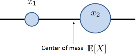
\E[X] = (1) p_X(1) + (0) p_X(0) = (1)\left(\frac{3}{4}\right) + (0)\left(\frac{1}{4}\right) = \frac{3}{4}.

Center of mass. How would you interpret the result of this example? Does it mean that, on average, we will get $3/4$ heads (but there is not anything called $3/4$ heads!). Recall the definition of a random variable: it is a translator that translates a descriptive state to a number on the real line. Thus the expectation, which is an operation defined on the real line, can only tell us what is happening on the real line, not in the original sample space. On the real line, the expectation can be regarded as the center of mass, which is the point where the “forces” between the two states are “balanced”. In Figure 3.16 we depict a random variable with two states $x_1$ and $x_2$. The state $x_1$ has less influence (because $p_X(x_1)$ is smaller) than $x_2$. Therefore the center of mass is shifted towards $x_2$. This result shows us that the value $\E[X]$ is not necessarily in the sample space. $\E[X]$ is a deterministic number with nothing to do with the sample space.

**Figure 3.16.** Center of mass. If a state $x_2$ is more influential than another state $x_1$, the center of mass $\E[X]$ will lean towards $x_2$.

Example 3.12

Let $X$ be a random variable with PMF $p_X(k) = \frac{1}{2^k}$, for $k = 1,2,3,\ldots$. The expectation is

\begin{aligned} \E[X] = \sum_{k=1}^{\infty} k p_X(k) &= \sum_{k=1}^{\infty} k \cdot \frac{1}{2^k} \\ &= \frac{1}{2}\sum_{k=1}^{\infty} k \cdot \frac{1}{2^{k-1}} = \frac{1}{2} \cdot \frac{1}{(1-\frac{1}{2})^2} = 2. \end{aligned}

On MATLAB and Python, if you want to verify this answer you can use the following code. Here, we approximate the infinite sum by a finite sum of $k = 1, \ldots, 100$.

MATLAB

% MATLAB code to compute the expectation
    k = 1:100;
    p = 0.5.^k;
    EX = sum(p.*k);

Python

# Python code to compute the expectation
    import numpy as np
    k = np.arange(100)
    p = np.power(0.5,k)
    EX = np.sum(p*k)

Example 3.13

Roll a die twice. Let $X$ be the first roll and $Y$ be the second roll. Let $Z = \max(X,Y)$. To compute the expectation $\E[Z]$, we first construct the sample space. Since there are two rolls, we can construct a table listing all possible pairs of outcomes. This will give us $\{(1,1),(1,2), \ldots, (6,6)\}$. Now, we calculate $Z$, which is the max of the two rolls. So if we have $(1,3)$, then the max will be $3$, whereas if we have $(5,2)$, then the max will be 5. We can complete a table as shown below.

	1	2	3	4	5	6
1	1	2	3	4	5	6
2	2	2	3	4	5	6
3	3	3	3	4	5	6
4	4	4	4	4	5	6
5	5	5	5	5	5	6
6	6	6	6	6	6	6

This table tells us that $Z$ has 6 states. The PMF of $Z$ can be determined by counting the number of times a state shows up in the table. Thus, we can show that

\begin{aligned} p_Z(1) &= \frac{1}{36}, \; p_Z(2) = \frac{3}{36}, \; p_Z(3) = \frac{5}{36}, \\ &\qquad \; p_Z(4) = \frac{7}{36}, \; p_Z(5) = \frac{9}{36}, \; p_Z(6) = \frac{11}{36}. \end{aligned}

The expectation of $Z$ is therefore

\begin{aligned} \E[Z] &= (1)\left(\frac{1}{36}\right) + (2)\left(\frac{3}{36}\right) + (3)\left(\frac{5}{36}\right) \\ &\qquad + (4)\left(\frac{7}{36}\right) + (5)\left(\frac{9}{36}\right) + (6)\left(\frac{11}{36}\right) \\ &= \frac{161}{36}. \end{aligned}

Example 3.14

Consider a game in which we flip a coin 3 times. The reward of the game is

$1 if there are 2 heads
$8 if there are 3 heads
$0 if there are 0 or 1 head

There is a cost associated with the game. To enter the game, the player has to pay $1.50. We want to compute the net gain, on average.

To answer this question, we first note that the sample space contains 8 elements: HHH, HHT, HTH, THH, THT, TTH, HTT, TTT. Let $X$ be the number of heads. Then the PMF of $X$ is

\begin{aligned} p_X(0) = \frac{1}{8}, \;\; p_X(1) = \frac{3}{8}, \;\; p_X(2) = \frac{3}{8}, \;\; p_X(3) = \frac{1}{8}. \end{aligned}

We then let $Y$ be the reward. The PMF of $Y$ can be found by “adding” the probabilities of $X$. This yields

\begin{aligned} p_Y(0) = p_X(0) + p_X(1) = \frac{4}{8}, \;\; p_Y(1) = p_X(2) = \frac{3}{8}, \;\; p_Y(8) = p_X(3) = \frac{1}{8}. \end{aligned}

The expectation of $Y$ is

\E[Y] = (0)\left(\frac{4}{8}\right) + (1)\left(\frac{3}{8}\right) + (8)\left(\frac{1}{8}\right) = \frac{11}{8}.

Since the cost of the game is $\frac{12}{8}$, the net gain (on average) is $-\frac{1}{8}$.

3.4.2Existence of expectation

Does every PMF have an expectation? No, because we can construct a PMF such that the expectation is undefined.

Example 3.15

Consider a random variable $X$ with the following PMF:

p_X(k) = \frac{6}{\pi^2 k^2}, \quad\quad k = 1, 2, \ldots.

Using a result from algebra, one can show that $\sum_{k=1}^{\infty}\frac{1}{k^2} = \frac{\pi^2}{6}$. Therefore, $p_X(k)$ is a legitimate PMF because $\sum_{k=1}^{\infty}p_X(k) = 1$. However, the expectation diverges, because

\begin{aligned} \E[X] &= \sum_{k=1}^{\infty} k p_X(k) \\ &= \frac{6}{\pi^2} \sum_{k=1}^{\infty} \frac{1}{k} \rightarrow \infty, \end{aligned}

where the divergence is due to the harmonic series (https://en.wikipedia.org/wiki/Harmonic_series_(mathematics)): $1+\frac{1}{2}+\frac{1}{3}+\cdots = \infty$.

A PMF has an expectation when it is absolutely summable.

Definition 3.5

A discrete random variable $X$ is absolutely summable if

\E[|X|] \bydef \sum_{x\in X(\Omega)} |x| \; p_X(x) < \infty.

This definition tells us that not all random variables have a finite expectation. This is a very important mathematical result, but its practical implication is arguably limited. Most of the random variables we use in practice are absolutely summable. Also, note that the property of absolute summability applies to discrete random variables. For continuous random variables, we have a parallel concept called absolute integrability, which will be discussed in the next chapter.

3.4.3Properties of expectation

The expectation of a random variable has several useful properties. We list them below. Note that these properties apply to both discrete and continuous random variables.

Theorem 3.4

The expectation of a random variable $X$ has the following properties:

(i)
Function. For any function $g$, $$\E[g(X)] = \sum_{x \in X(\Omega)} g(x)\; p_X(x).$$
(ii)
Additive. For any function $g$ and $h$, $$\E[g(X) + h(X)] = \E[g(X)] + \E[h(X)].$$
(iii)
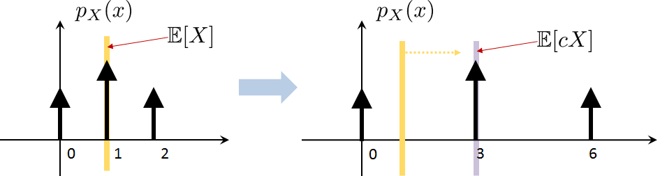
Scale. For any constant $c$, $$\E[cX] = c\E[X].$$
(iv)
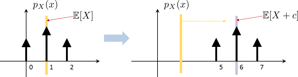
DC Shift. For any constant $c$, $$\E[X+c] = \E[X]+c.$$

Proof of (i). A pictorial proof of (i) is shown in Figure 3.17. The key idea is a change of variable.

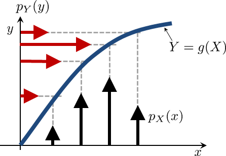
When we have a function $Y = g(X)$, the PMF of $Y$ will have impulses moved from $x$ (the horizontal axis) to $g(x)$ (the vertical axis). The PMF values (i.e., the probabilities or the height of the stems), however, are not changed. If the mapping $g(X)$ is many-to-one, multiple PMF values will add to the same position. Therefore, when we compute $\E[g(X)]$, we compute the expectation along the vertical axis.

■

Practice Exercise 3.3

Prove statement (iii): For any constant $c$, $\E[cX] = c\E[X]$.

Solution

Recall the definition of expectation:

\begin{aligned} \E[cX] &= \sum_{x \in X(\Omega)} (cx) p_X(x) = c \;\; \underset{\textcolor{blue}{=\E[X]}}{\underbrace{\sum_{x \in X(\Omega)} x p_X(x)}} = c\E[X]. \end{aligned}

Statement (iii) is illustrated in Figure 3.18. Here, we assume that the original PMF has 3 states $X = 0,1,2$. We multiply $X$ by a constant $c = 3$. This changes $X$ to $cX = 0, 3, 6$. However, since the probabilities are not changed, the height of the PMF values remains. Therefore, when computing the expectation, we just multiply $\E[X]$ by $c$ to get $c\E[X]$.

Practice Exercise 3.4

Prove statement (ii): For any function $g$ and $h$, $\E[g(X) + h(X)] = \E[g(X)] + \E[h(X)].$

Solution

Recall the definition of expectation:

\begin{aligned} \E[g(X)+h(X)] &= \sum_{x \in X(\Omega)} [g(x)+h(x)] p_X(x) \\ &= \underset{\textcolor{blue}{=\E[g(X)]}}{\underbrace{\sum_{x \in X(\Omega)} g(x) p_X(x)}} + \underset{\textcolor{blue}{=\E[h(X)]}}{\underbrace{\sum_{x \in X(\Omega)} h(x) p_X(x)}}\\ &= \E[g(X)] + \E[h(X)]. \end{aligned}

Practice Exercise 3.5

Prove statement (iv): For any constant $c$, $\E[X+c] = \E[X]+c$.

Solution

Recall the definition of expectation:

\begin{aligned} \E[X+c] &= \sum_{x \in X(\Omega)} (x+c) p_X(x) \\ &= \underset{\textcolor{blue}{=\E[X]}}{\underbrace{\sum_{x \in X(\Omega)} x p_X(x)}} + c \cdot \underset{\textcolor{blue}{=1}}{\underbrace{\sum_{x \in X(\Omega)} p_X(x)}} \\ &= \E[X]+c. \end{aligned}

This result is illustrated in Figure 3.19. As we add a constant to the random variable, its PMF values remain the same but their positions are shifted. Therefore, when computing the mean, the mean will be shifted accordingly.

Example 3.16

Let $X$ be a random variable with four equally probable states $0, 1, 2, 3$. We want to compute the expectation $\E[\cos(\pi X/2)]$. To do so, we note that

\begin{aligned} \E[\cos(\pi X /2)] &= \sum_{x \in X(\Omega)} \cos \left(\frac{\pi x}{2}\right) p_X(x) \\ &\hspace{-6ex}= (\cos 0) \left(\frac{1}{4}\right) + (\cos \frac{\pi}{2}) \left(\frac{1}{4}\right) + (\cos \frac{2 \pi}{2}) \left(\frac{1}{4}\right) + (\cos \frac{3\pi}{2}) \left(\frac{1}{4}\right) \\ &\hspace{-6ex}= \frac{1 + 0 + (-1) + 0}{4} = 0. \end{aligned}

Example 3.17

Let $X$ be a random variable with $\E[X] = 1$ and $\E[X^2] = 3$. We want to find the expectation $\E[(aX+b)^2]$. To do so, we realize that

\begin{aligned} \E[(aX+b)^2] &\overset{(a)}{=} \E[a^2 X^2 + 2ab X + b^2] \overset{(b)}{=} a^2\E[X^2] + 2ab \E[X] + b^2 = 3a^2 + 2ab + b^2, \end{aligned}

where $(a)$ is due to expansion of the square, and $(b)$ holds in two steps. The first step is to apply statement (ii) for individual functions of expectations, and the second step is to apply statement (iii) for scalar multiple of the expectations.

3.4.4Moments and variance

Based on the concept of expectation, we can define a moment:

Definition 3.6

The $k$th moment of a random variable $X$ is

\E[X^k] = \sum_{x}\, x^k \, p_X(x).

Essentially, the $k$th moment is the expectation applied to $X^k$. The definition follows from statement (i) of the expectation's properties. Using this definition, we note that $\E[X]$ is the first moment and $\E[X^2]$ is the second moment. Higher-order moments can be defined, but in practice they are less commonly used.

Example 3.18

Flip a coin 3 times. Let $X$ be the number of heads. Then

\begin{aligned} p_X(0) = \frac{1}{8}, \;\; p_X(1) = \frac{3}{8}, \;\; p_X(2) = \frac{3}{8}, \;\; p_X(3) = \frac{1}{8}. \end{aligned}

The second moment $\E[X^2]$ is

\begin{aligned} \E[X^2] = (0)^2\left(\frac{1}{8}\right) + (1)^2\left(\frac{3}{8}\right) + (2)^2\left(\frac{3}{8}\right) + (3)^2\left(\frac{1}{8}\right) = 3. \end{aligned}

Example 3.19

Consider a random variable $X$ with PMF

\begin{aligned} p_X(k) = \frac{1}{2^k}, \quad\quad k = 1,2,\ldots. \end{aligned}

The second moment $\E[X^2]$ is

\begin{aligned} \E[X^2] = \sum_{k=1}^{\infty} k^2 \left(\frac{1}{2}\right)^k &= \textcolor{red}{\frac{1}{2^2}} \sum_{k=1}^{\infty} k(k\textcolor{blue}{-1+1}) \left(\frac{1}{2}\right)^{k\textcolor{red}{-2}} \\ &= \frac{1}{2^2} \sum_{k=1}^{\infty} k(k\textcolor{blue}{-1}) \left(\frac{1}{2}\right)^{k\textcolor{red}{-2}} + \frac{1}{2^2} \sum_{k=1}^{\infty} k \left(\frac{1}{2}\right)^{k\textcolor{red}{-2}}\\ &= \frac{1}{2^2} \left(\frac{2}{(1-\frac{1}{2})^3}\right) + \frac{1}{2} \left( \frac{1}{(1-\frac{1}{2})^2}\right) = 6. \end{aligned}

Using the second moment, we can define the variance of a random variable.

Definition 3.7

The variance of a random variable $X$ is

\Var[X] = \E[(X-\mu)^2],

where $\mu = \E[X]$ is the expectation of $X$.

We denote $\sigma^2$ by $\Var[X]$. The square root of the variance, $\sigma$, is called the standard deviation of $X$. Like the expectation $\E[X]$, the variance $\Var[X]$ is computed using the ideal histogram PMF. It is the limiting object of the usual standard deviation we calculate from a dataset.

On a computer, computing the variance of a dataset is done by calling built-in commands such as var in MATLAB and np.var in Python. The standard deviation is computed using std and np.std, respectively.

MATLAB

% MATLAB code to compute the variance
    X = rand(10000,1);
    vX = var(X);
    sX = std(X);

Python

% Python code to compute the variance
    import numpy as np
    X = np.random.rand(10000)
    vX = np.var(X)
    sX = np.std(X)

What does the variance mean? It is a measure of the deviation of the random variable $X$ relative to its mean. This deviation is quantified by the squared difference $(X-\mu)^2$. The expectation operator takes the average of the deviation, giving us a deterministic number $\E[(X-\mu)^2]$.

Theorem 3.5

The variance of a random variable $X$ has the following properties:

(i)
Moment. $$\Var[X] = \E[X^2] - \E[X]^2.$$
(ii)
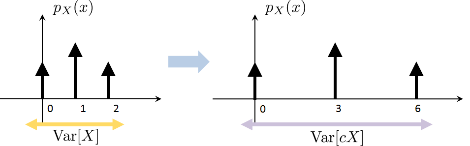
Scale. For any constant $c$, $$\Var[cX] = c^2\Var[X].$$
(iii)
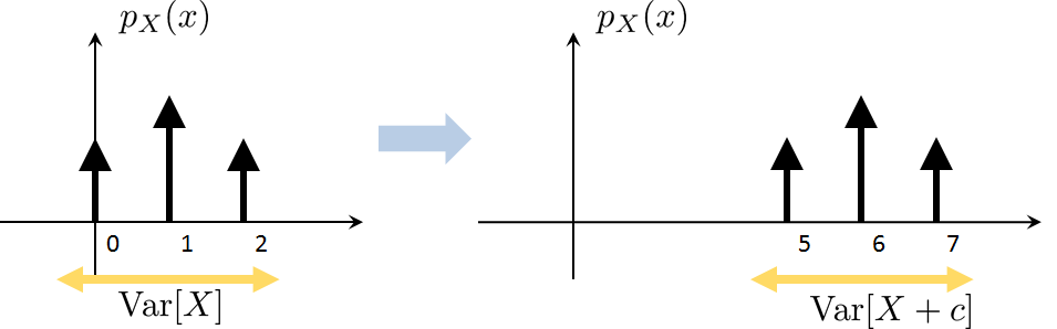
DC Shift. For any constant $c$, $$\Var[X+c] = \Var[X].$$

**Figure 3.20.** Pictorial representations of $\Var[cX] = c^2\Var[X]$ and $\Var[X+c] = \Var[X]$.

Practice Exercise 3.6

Prove Theorem def:variance property above.

Solution

For statement (i), we show that

\begin{aligned} \Var[X] = \E[(X-\mu)^2] &= \E[X^2 - 2X\mu + \mu^2] = \E[X^2] - \mu^2. \end{aligned}

Statement (ii) holds because $\E[cX] = c\mu$ and

\begin{aligned} \Var[cX] &= \E[(cX-\E[cX])^2] \\ &= \E[(cX - c\mu)^2] = c^2\E[(X-\mu)^2] = c^2\Var[X]. \end{aligned}

Statement (iii) holds because

\begin{aligned} \Var[X+c] &= \E[((X+c)-\E[X+c])^2] = \E[(X-\E[X])^2] = \Var[X]. \end{aligned}

The properties above are useful in various ways. The first statement provides a link connecting variance and the second moment. Statement (ii) implies that when $X$ is scaled by $c$, the variance should be scaled by $c^2$ because of the square in the second moment. Statement (iii) says that when $X$ is shifted by a scalar $c$, the variance is unchanged. This is true because no matter how we shift the mean, the fluctuation of the random variable remains the same.

Practice Exercise 3.7

Flip a coin with probability $p$ to get a head. Let $X$ be a random variable denoting the outcome. The PMF of $X$ is

\begin{aligned} p_X(0) = 1-p, \quad\quad p_X(1) = p. \end{aligned}

Find $\E[X]$, $\E[X^2]$ and $\Var[X]$.

Solution

The expectation of $X$ is

\begin{aligned} \E[X] = (0)p_X(0) + (1)p_X(1) = (0)(1-p) + (1)(p) = p. \end{aligned}

The second moment is

\begin{aligned} \E[X^2] = (0)^2p_X(0) + (1)^2p_X(1) = p. \end{aligned}

The variance is

\begin{aligned} \Var[X] &= \E[X^2] - \E[X]^2 = p - p^2 = p(1-p). \end{aligned}