Wide-Sense Stationary Processes

As we have seen in the previous sections, some random processes have a “nice” autocorrelation function, in the sense that the 2D function \(R_X(t_1,t_2)\) has a Toeplitz structure. Random processes with this property are known as wide-sense stationary (WSS) processes. WSS processes belong to a very small subset in the entire universe of random processes, but they are practically the most useful ones. Before we discuss how to use them, we first present a formal definition of a WSS process. (Many textbooks introduce strictly stationary processes before discussing a wide-sense stationary process. We skip the former because, throughout our book, we only use WSS processes. Readers interested in strictly stationary processes can consult the references listed at the end of this chapter.)

10.3.1Definition of a WSS process

There are two criteria that define a WSS process. The first criterion is that the mean is a constant. That is, the mean function does not change with time. The second criterion is that the autocorrelation function only depends on the difference \(t_1-t_2\) and not on the absolute starting point. For example, \(R_X(0.1,1.1)\) needs to be the same as \(R_X(6.3,7.3)\), because the intervals are both 1.

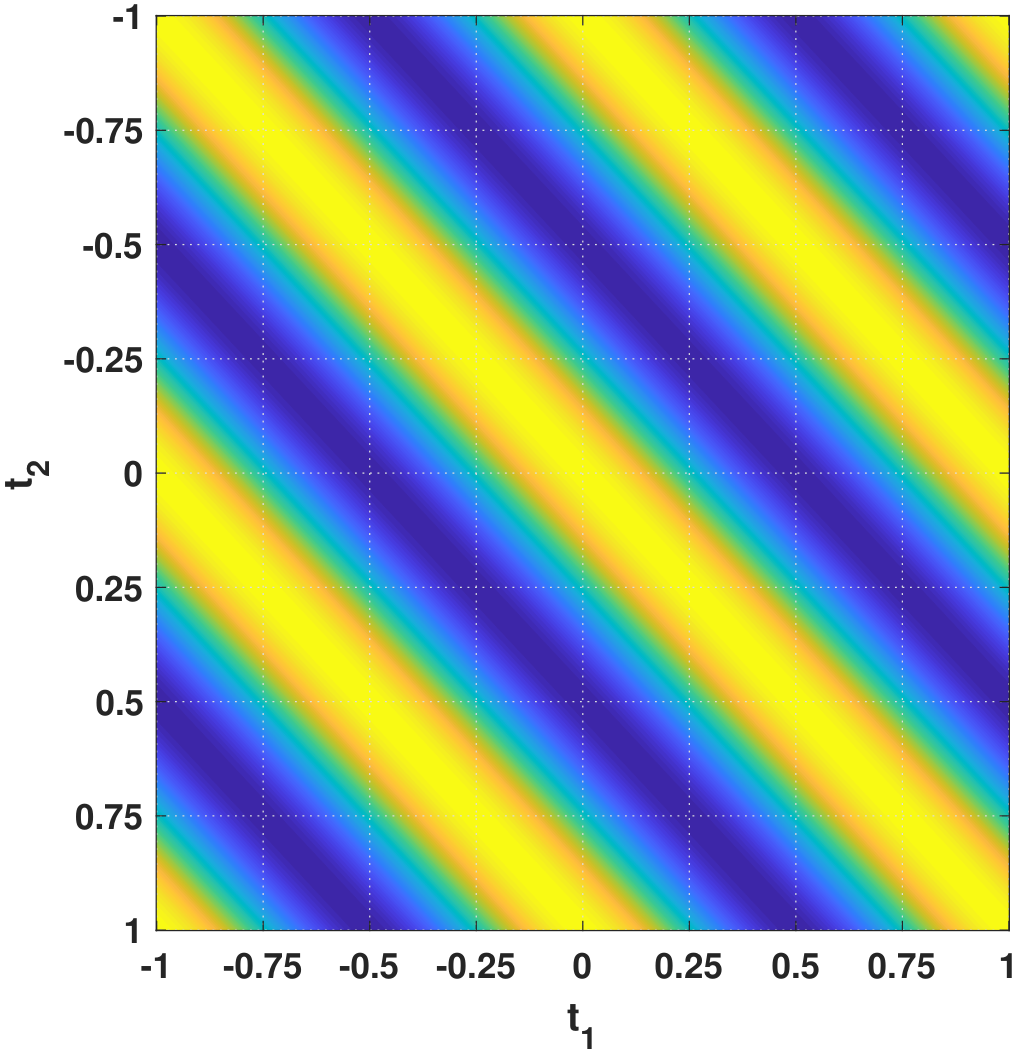
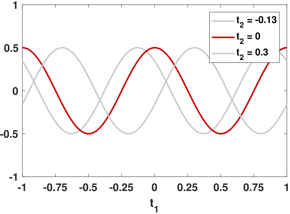
How can these two criteria be mapped to the Toeplitz structure we discussed in the previous examples? Figure 10.14 shows the autocorrelation function \(R_X(t_1,t_2)\), which is a 2D function. We take three cross sections corresponding to \(t_2 = -0.13\), \(t_2 = 0\) and \(t_2 = 0.3\). As you can see from the figure, each \(R_X(t_1, t_2)\) is a shifted version of another one. To obtain any value \(R_X(t_1,t_2)\) on the function, there is no need to probe to the 2D map; you only need to probe to the red curve and locate the position marked as \(t_1 - t_2\), and you will be able to obtain the value \(R_X(t_1,t_2)\).

Not all random processes have a Toeplitz autocorrelation function. For example, the random process \(X(t) = A\cos(2\pi t)\) is not a WSS process, because the autocorrelation function is

which cannot be written as the difference \(t_1-t_2\).

Remark 1. WSS processes can also be defined using the autocovariance function instead of the autocorrelation function, because if a process is WSS, then the mean function is a constant. If the mean function is a constant, then \(C_X(t_1,t_2) = R_X(t_1,t_2) - \mu^2\). So any geometric structure that \(R_X\) possesses will be translated to \(C_X\), as the constant \(\mu^2\) will not influence the geometry. Therefore, it is equally valid to say that a WSS process has

Remark 2. Because a WSS is completely characterized by the difference \(t_1-t_2\), there is no need to keep track of the absolute indices \(t_1\) and \(t_2\). We can rewrite the autocorrelation function as

There is nothing new in this equation: It only says that instead of writing \(R_X(t+\tau,t)\), we can write \(R_X(\tau)\) because the time index \(t\) plays no role in terms of \(R_X\). Thus from now on, for any WSS processes we will write the autocorrelation function as \(R_X(\tau)\).

10.3.2Properties of \(R_X(\tau)\)

When \(X(t)\) is WSS, \(R_X(\tau)\) has several important properties.

This result says that if \(R_X(\tau)\) is slowly decaying from \(R_X(0)\), the probability of having a large deviation \(|X(t+\tau)-X(t)|\) is small.

10.3.3Physical interpretation of \(R_X(\tau)\)

How should we understand the autocorrelation function \(R_X(\tau)\) for WSS processes? Certainly, by definition, \(R_X(\tau) = \E[X(t+\tau)X(t)]\) means that we can analyze \(R_X(\tau)\) from the statistical perspective. But in this section we want to take a slightly different approach by answering the question from a computational perspective.

Consider the following function:

This function is the temporal average of \(X(t+\tau)X(t)\), as opposed to the statistical average. Why do we want to consider this temporal average? We first show the main result, that \(\E[\widehat{R}_X(\tau)] = R_X(\tau)\).

This lemma implies that if the signal \(X(t)\) is long enough, we can approximate \(R_X(\tau)\) by \(\widehat{R}_X(\tau)\). The approximation is asymptotically consistent, in the sense that \(\E[\widehat{R}_X(\tau)] = R_X(\tau)\). Now, the more interesting question is the interpretation of \(\widehat{R}_X(\tau)\). What is it?

Correlation is analogous to convolution. For convolution, the definition is

whereas for correlation, the definition is

Clearly, \(\widehat{R}_X(\tau)\) is the latter. A graphical illustration of the difference between convolution and correlation is provided in Figure 10.15. The only difference between the two is that the correlation does not flip the function, whereas the convolution does flip the function.

The temporal correlation is easy to visualize. Starting with the function \(X(t+\tau)\), if you make \(\tau\) larger or smaller, then effectively you are shifting \(X(t)\) left or right. The integration \(\int_{-T}^T X(t+\tau)X(t)\;dt\) calculates the energy accumulated. If the integral is large, there is a strong correlation between \(X(t)\) and \(X(t+\tau)\). Otherwise the correlation is small. Here is an extreme example:

Example 10.14

Consider a random process \(X(t)\) such that for every \(t\), \(X(t)\) is an i.i.d. Gaussian random variable with zero mean and unit variance. Then

$$\begin{aligned} R_X(\tau) = \E[X(t+\tau)X(t)] &= \begin{cases} \E[X^2(t)], &\qquad \tau = 0,\\ \E[X(t+\tau)]\E[X(t)], &\qquad \tau \not= 0. \end{cases} \end{aligned}$$

Using the fact that \(X(t)\) is i.i.d. Gaussian for all \(t\), we can show that \(\E[X^2(t)] = 1\) for any \(t\), and \(\E[X(t+\tau)]\E[X(t)] = 0\). Therefore, we have

$$\begin{aligned} R_X(\tau) = \begin{cases} 1, &\qquad \tau = 0,\\ 0, &\qquad \tau \not= 0. \end{cases} \end{aligned}$$

The equation says that since the random process is i.i.d. Gaussian, shifting and integrating will give maximum correlation at the origin. As soon as the shift is not at the origin, the correlation is zero. This makes sense because the samples are just i.i.d. Gaussian. One pixel offset is enough to destroy any correlation.

Now let's calculate the temporal correlation. We know that

$$\begin{aligned} \widehat{R}_X(\tau) = \frac{1}{2T}\int_{-T}^T X(t+\tau)X(t) \;dt. \end{aligned}$$

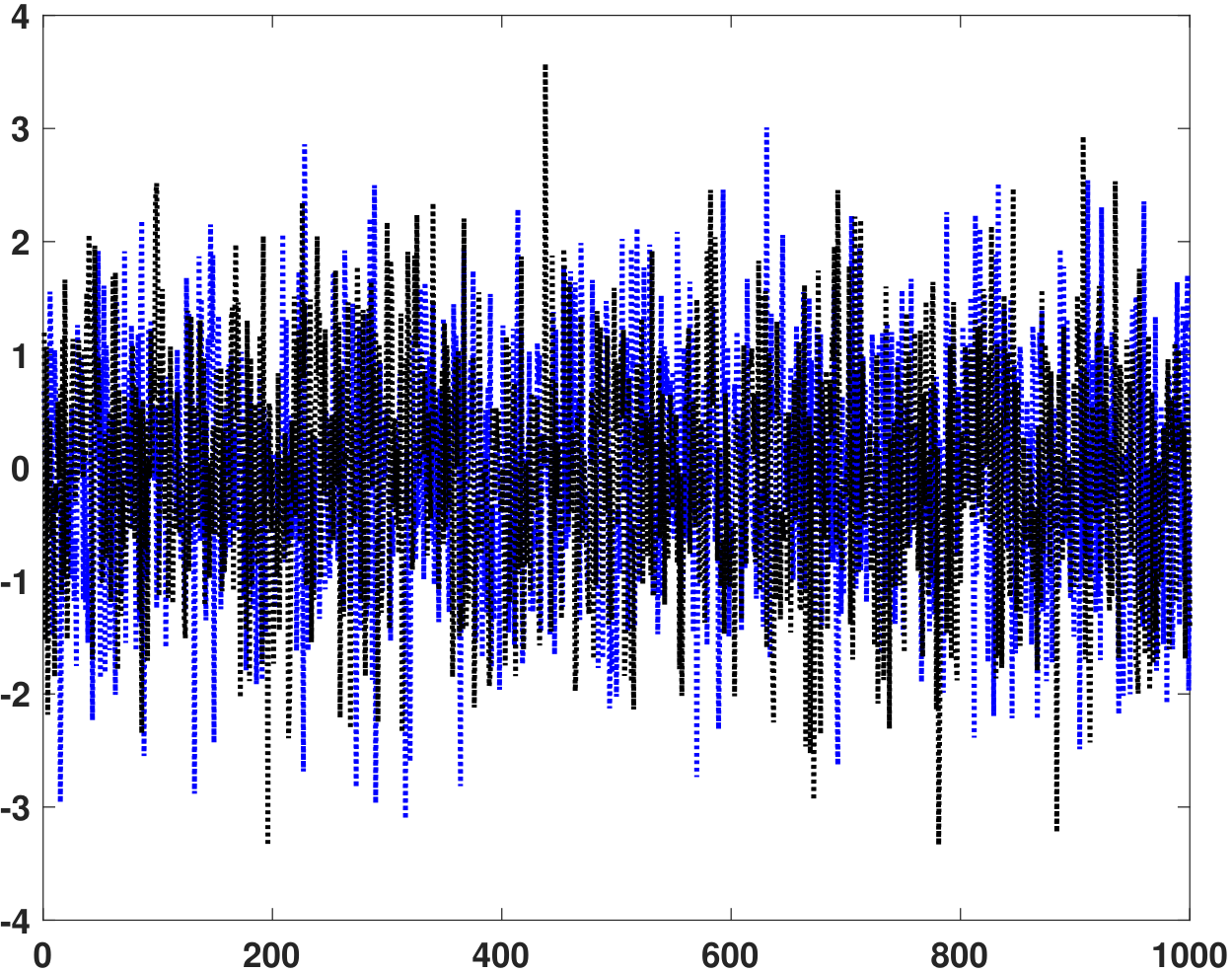
This equation says that we shift \(X(t)\) to the left and right and then integrate. If \(\tau\) is not zero, the product \(X(t+\tau)X(t)\) will sometimes be positive and sometimes be negative. After integrating the entire period, we cancel out most of the terms. Let's plot the functions and see if all of these steps make sense. In Figure 10.16(a), we show two random realizations of the random process \(X(t)\). They are just i.i.d. Gaussian samples.

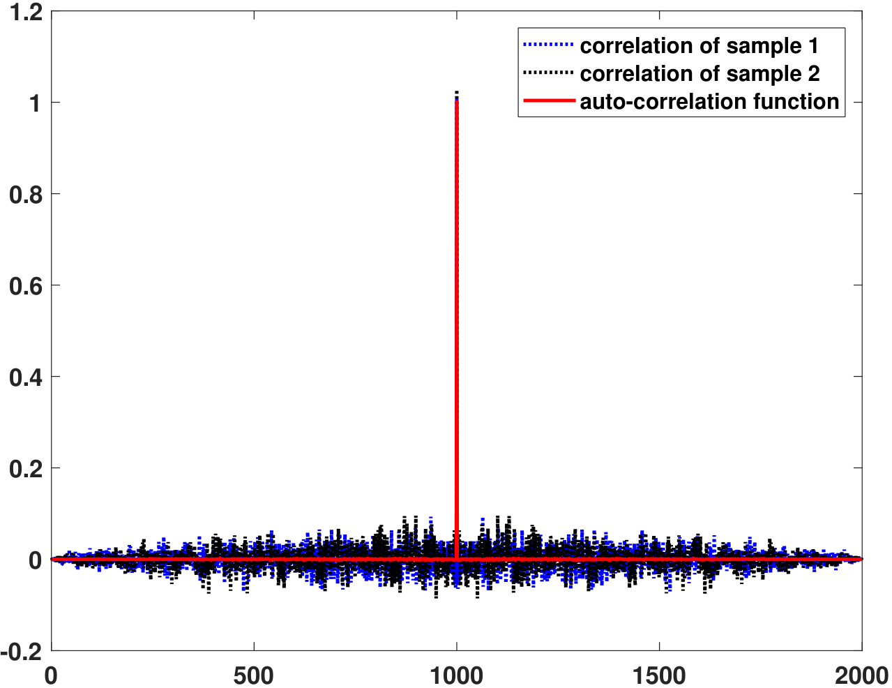
In Figure 10.16(b) we plot the temporal autocorrelation function \(\widehat{R}_X(\tau)\). Since \(\widehat{R}_X(\tau)\) itself is a random process, it has different realizations. We plot two random realizations, which are computed based on shifting and integrating \(X(t)\). In the same plot, we also show the statistical expectation \(R_X(\tau)\). As we can see from the plot, the temporal correlation and the statistical correlation match reasonably well except for the fluctuation in \(\widehat{R}_X(\tau)\), which is expected because it is computed from a finite number of samples.

On a computer, the commands to do the autocorrelation function are xcorr in MATLAB and np.correlate in Python. Below are the codes used to generate Figure 10.16.

% MATLAB code to demonstrate autocorrelation
    N     = 1000; % number of sample paths
    T     = 1000; % number of time stamps
    X     = 1*randn(N,T);
    xc    = zeros(N,2*T-1);
    
    for i=1:N
        xc(i,:) = xcorr(X(i,:))/T;
    end
    plot(xc(1,:),'b:', 'LineWidth', 2); hold on;
    plot(xc(2,:),'k:', 'LineWidth', 2);

# Python code to demonstrate autocorrelation
    N = 1000
    T = 1000
    X = np.random.randn(N,T)
    xc= np.zeros((N,2*T-1))
    
    for i in range(N):
      xc[i,:] = np.correlate(X[i,:],X[i,:],mode='full')/T
    plt.plot(xc[0,:],'b:')
    plt.plot(xc[1,:],'k:')
    plt.show()

Under what conditions will \(\widehat{R}_X(\tau) \rightarrow R_X(\tau)\) as \(T \rightarrow \infty\)? The answer to this question is provided by an important theorem called Mean-Square Ergodic Theorem, which can be thought of as the random process version of the weak law of large numbers. We leave the discussion of the mean-square ergodic theorem to the Appendix.