eBook › Chapter 10 · Random Processes

Section 10.5

WSS Process through LTI Systems

Random processes have limited usefulness until we can apply operations to them. In this section we discuss how WSS processes respond to a linear time-invariant (LTI) system. This technique is most useful in signal processing, communication, speech analysis, and imaging. We will be brief here since you can find most of this information in any standard textbook on signals and systems.

10.5.1Review of linear time-invariant systems

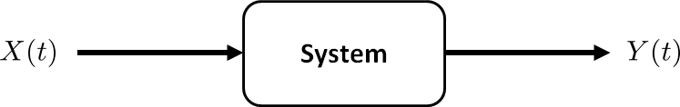
When we say a “system”, we mean that there exists an input-output relationship as shown in Figure 10.21.

Linear time-invariant (LTI) systems are the simplest systems we use in engineering problems. An LTI system has two properties.

Linearity. Linearity means that when two input random processes are added and scaled, the output random processes will also be added and scaled in exactly the same way. Mathematically, linearity says that if $X_1(t) \rightarrow Y_1(t)$ and $X_2(t) \rightarrow Y_2(t)$, then $$aX_1(t)+bX_2(t) \rightarrow a Y_1(t) + b Y_2(t).$$
Time-invariant: Time invariance means that if we shift the input random process by a certain time period, the output will be shifted in the same way. Mathematically, time invariance means that if $X(t) \rightarrow Y(t)$, then $$X(t+\tau) \rightarrow Y(t+\tau).$$

If a system is linear time-invariant, the input-to-output relation is given by convolution:

The convolution between two functions $X(t)$ and $h(t)$ is defined as

\begin{aligned} Y(t) = h(t) \ast X(t) &= \int_{-\infty}^{\infty} h(\tau)\;X(t-\tau)\;d\tau, \end{aligned}

in which we call $h(t)$ the system response or impulse response.

The function $h(t)$ is called the impulse response because if $X(t) = \delta(t)$, then according to the convolution equation we have

Y(t) = \int_{-\infty}^{\infty} h(\tau)\;\delta(t-\tau)\;d\tau = h(t).

Therefore, if we send an impulse to the system, the output will be $h(t)$.

Convolution is commutative, meaning that $h(t) \ast X(t) = X(t) \ast h(t)$. Written as integrations, we have

\int_{-\infty}^{\infty} h(\tau)\;X(t-\tau)\;d\tau = \int_{-\infty}^{\infty} h(t-\tau)\;X(\tau)\;d\tau.

For LTI systems, $Y(t)$ can be determined through the Fourier transforms.

The Fourier transform of a (square-integrable) function $X(t)$ is

X(\omega) = \calF\{X(t)\} = \int_{-\infty}^{\infty} X(\tau)\; e^{-j \omega \tau }\;d\tau.

A basic property of convolution is that convolution in the time domain is equivalent to multiplication in the Fourier domain. Therefore

Y(\omega) = H(\omega)X(\omega),

where $H(\omega) = \calF\{h(t)\}$ is the Fourier transform of $h(t)$, and $Y(\omega) = \calF(Y(t))$ is the Fourier transform of $Y(t)$.

In the rest of this section we study the pair of input and output random processes that are defined as follows

sep0ex
$X(t)$ = input. It is a WSS random process.
$Y(t)$ = output. It is constructed by sending $X(t)$ through an LTI system with impulse response $h(t)$. Therefore, $Y(t) = h(t)\ast X(t)$.

10.5.2Mean and autocorrelation through LTI Systems

Since $X(t)$ is WSS, the mean function of $X(t)$ stays constant, i.e., $\mu_X(t) = \mu_X$. The following theorem gives the mean function of the output.

Theorem 10.3

If $X(t)$ passes through an LTI system to yield $Y(t)$, the mean function of $Y(t)$ is

\E[Y(t)]=\mu_X \int_{-\infty}^{\infty}h(\tau) \;d\tau.

Proof. Suppose that $Y(t) = h(t) \ast X(t)$. Then,

\begin{aligned} \mu_Y(t) =\E[Y(t)] &=\E\left[\int_{-\infty}^{\infty}h(\tau)X(t-\tau)\;d\tau\right] \\ &= \int_{-\infty}^{\infty}h(\tau)\E[X(t-\tau)]\;d\tau\\ &= \int_{-\infty}^{\infty}h(\tau) \mu_X\; d\tau = \mu_X \int_{-\infty}^{\infty}h(\tau)\; d\tau, \end{aligned}

where the second-to-last equality is valid because $\E[X(t-\tau)]=\mu_X$.

■

The theorem suggests that if the input $X(t)$ has a constant mean, the output $Y(t)$ should also have a constant mean. This should not be a surprise because if the system is linear, a constant input will give a constant output.

Example 10.15

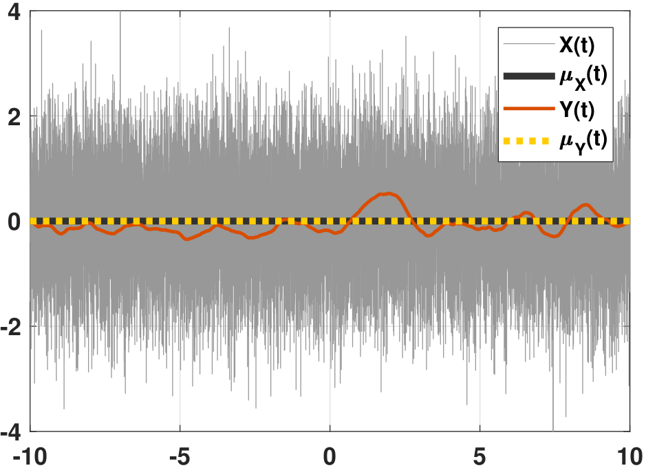
Consider a WSS random process $X(t)$ such that each sample is an i.i.d. Gaussian random variable with zero mean and unit variance. We send this process through an LTI system with impulse response $h(t)$, where

h(t) = \begin{cases} 10(1-|t|), &\;\; -1 \le t \le 1,\\ 0, &\;\; \text{otherwise}. \end{cases}

The mean function of $X(t)$ is $\mu_X(t) = 0$, and that of $Y(t)$ is $\mu_Y(t) = 0$. Figure 10.22 illustrates a numerical example, in which we see that the random processes $X(t)$ and $Y(t)$ have different shapes but the mean functions remain constant.

**Figure 10.22.** When sending a WSS random process through an LTI system, the mean and the autocorrelation functions are changed.

Next, we derive the autocorrelation function of a random process when sent through an LTI system.

Theorem 10.4

If $X(t)$ passes through an LTI system to yield $Y(t)$, the autocorrelation function of $Y(t)$ is

R_Y(\tau)=\int_{-\infty}^{\infty}\int_{-\infty}^{\infty} h(s)h(r)R_X(\tau+s-r)\;ds\;dr.

Proof. We start with the definition of $Y(t)$:

\begin{aligned} R_Y(\tau)=\E[Y(t)Y(t+\tau)] &= \E\left[\int_{-\infty}^{\infty} h(s) X(t-s) \;ds \int_{-\infty}^{\infty} h(r)X(t+\tau-r)\;dr\right] \\ &\overset{(a)}{=} \int_{-\infty}^{\infty}\int_{-\infty}^{\infty} h(s)h(r)\E\left[X(t-s)X(t+\tau-r)\right]\;ds\;dr \\ &= \int_{-\infty}^{\infty}\int_{-\infty}^{\infty} h(s)h(r)R_X(\tau+s-r)\;ds\;dr, \end{aligned}

where in (a) we assume that integration and expectation are interchangeable.

■

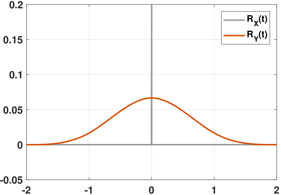
A shorthand notation of the above formula is $R_Y(t) = [h \circledast (h \ast R_X)](t)$, where $\ast$ denotes the convolution and $\circledast$ denotes the correlation. Figure 10.22(b) shows the autocorrelation functions $R_X$ and $R_Y$. In this example $R_X$ is a delta function because for i.i.d. Gaussian noise the power spectral density is a constant. After convolving with the system response, the autocorrelation $R_Y$ has a different shape.

10.5.3Power spectral density through LTI systems

Denoting the Fourier transform of the impulse response by $H(\omega) = \calF(h(t))$, we derive the power spectral density of the output.

Theorem 10.5

If $X(t)$ passes through an LTI system to yield $Y(t)$, the power spectral density of $Y(t)$ is

S_Y(\omega) = |H(\omega)|^2S_X(\omega).

Proof. By definition, the power spectral density $S_Y(\omega)$ is the Fourier transform of the autocorrelation function $R_Y(\tau)$. Therefore,

\begin{aligned} S_Y(\omega) &=\int_{-\infty}^{\infty}R_Y(\tau) e^{-j \omega \tau}\; d\tau\\ &=\int_{-\infty}^{\infty}\int_{-\infty}^{\infty}\int_{-\infty}^{\infty}h(s)h(r)R_X(\tau+s-r)\;ds\;dr e^{-j \omega \tau} \;d\tau. \end{aligned}

Letting $u=\tau+s-r$, we have

\begin{aligned} S_Y(\omega)&=\int_{-\infty}^{\infty}\int_{-\infty}^{\infty}\int_{-\infty}^{\infty}h(s)h(r)R_X(u) e^{-j \omega (u-s+r)} \;ds\;dr\;du \\ &=\int_{-\infty}^{\infty} h(s)e^{j \omega s} \;ds \int_{-\infty}^{\infty} h(r)e^{-j \omega r} \;dr \int_{-\infty}^{\infty} R_X(u) e^{-j \omega u} \;du \\ &=\overline{H(\omega)} H(\omega) S_X(\omega), \end{aligned}

where $\overline{H(\omega)}$ is the complex conjugate of $H(\omega)$.

■

It is tempting to think that since $Y(t) = h(t)\ast X(t)$, the power spectral density should also be $S_Y(\omega) = H(\omega) X(\omega)$, but this is not true. The above result shows that we need an additional complex conjugate $\overline{H(\omega)}$ because $S_Y(\omega)$ is the power, which means the square of the signal. Note that $R_X$ is “squared” because we have convolved it with itself, and $R_Y$ is also squared. Therefore, to match $R_X$ and $R_Y$, the impulse response $h$ also needs to be squared in the Fourier domain.

Example 10.16

A WSS process $X(t)$ has a correlation function

R_X(\tau)=\mathrm{sinc}(\pi\tau).

Suppose that $X(t)$ passes through an LTI system with input/output relationship

2\frac{d^2}{dt^2}Y(t)+2\frac{d}{dt}Y(t)+4Y(t)=3\frac{d^2}{dt^2}X(t)-3\frac{d}{dt}X(t)+6X(t).

Find $R_Y(\tau)$.

Solution

: The sinc function has a Fourier transform given by

\mathrm{sinc}(Wt) \underset{\mathcal{F}}{\longleftrightarrow} \frac{\pi}{W}\mathrm{rect}\left(\frac{\omega}{2W}\right).

Therefore, the autocorrelation function is

R_X(\tau)=\mathrm{sinc}(\pi\tau) \quad \underset{\mathcal{F}}{\longleftrightarrow} \quad \frac{\pi}{\pi}\mathrm{rect}\left(\frac{\omega}{2\pi}\right).

By taking the Fourier transform on both sides, we have

S_X(\omega) = \begin{cases} 1,&\quad -\pi \leq \omega \leq \pi, \\ 0,&\quad \mbox{elsewhere}. \end{cases}

The system response is found from the differential equation:

\begin{aligned} H(\omega) &=\frac{3(j\omega)^2-3(j\omega)+6}{2(j\omega)^2+2(j\omega)+4} \\ &=\frac{3\left[(2-\omega^2)-j\omega\right]}{2\left[(2-\omega^2)+j\omega\right]}. \end{aligned}

Taking the magnitude square yields

\begin{aligned} |H(\omega)|^2 &=\frac{3\left[(2-\omega^2)-j\omega\right]}{2\left[(2-\omega^2)+j\omega\right]}\frac{3\left[(2-\omega^2)+j\omega\right]}{2\left[(2-\omega^2)-j\omega\right]} \\ &=\frac{9}{4} \frac{(2-\omega^2)^2+\omega^2}{(2-\omega^2)^2+\omega^2} =\frac{9}{4}. \end{aligned}

Therefore, the output power spectral density is

\begin{aligned} S_Y(\omega) &=|H(\omega)|^2S_X(\omega) =\frac{9}{4}S_X(\omega). \end{aligned}

Taking the inverse Fourier transform, we have

R_Y(\tau)=\frac{9}{4} \mathrm{sinc}(\pi\tau).

Example 10.17

A random process $X(t)$ has zero mean and $R_X(t,s)=\min(t,s)$. Consider a new process $Y(t)=e^t X(e^{-2t})$.

Is $Y(t)$ WSS?
Suppose $Y(t)$ passes through an LTI system to yield an output $Z(t)$ according to
$\frac{d}{dt}Z(t)+2Z(t)=\frac{d}{dt}Y(t)+Y(t).$
Find $R_Z(\tau)$.

Solution

In order to verify whether $Y(t)$ is WSS, we need to check the mean function and the autocorrelation function. The mean function is
$\begin{aligned} \E[Y(t)]&=\E\left[e^t X(e^{-2t})\right] = e^t \E\left[X(e^{-2t})\right]. \end{aligned}$
Since $X(t)$ has zero mean, $\E[X(t)]=0$ for all $t$. This implies that if $u=e^{-2t}$, then $\E[X(u)]=0$ because $u$ is just another time instant. Thus $\E[X(e^{-2t})]=0$, and hence $\E[Y(t)]=0$.

The autocorrelation is
$\begin{aligned} \E\left[Y(t+\tau)Y(t)\right]&=\E\left[e^{t+\tau}X(e^{-2(t+\tau)})e^t X(e^{-2t})\right] \\ &= e^{2t+\tau} \E\left[X(e^{-2(t+\tau)})X(e^{-2t})\right] \\ &= e^{2t+\tau} R_X(e^{-2(t+\tau)},e^{-2t}). \end{aligned}$
Substituting $R_X(t,s)=\min(t,s)$, we have that
$\begin{aligned} e^{2t+\tau} R_X(e^{-2(t+\tau)},e^{-2t}) &= e^{2t+\tau} \min(e^{-2(t+\tau)},e^{-2t}) \\ &= e^{2t+\tau} \left\{ \begin{array}{ll} e^{-2(t+\tau)}, & \tau \geq 0 \\ e^{-2t}, & \tau < 0 \\ \end{array} \right. \\ &= \left\{ \begin{array}{ll} e^{-\tau}, & \tau \geq 0 \\ e^{\tau}, & \tau < 0 \\ \end{array} \right. \\ &= e^{-|\tau|}. \end{aligned}$
So $R_Y(\tau)=e^{-|\tau|}$. Since $R_Y(\tau)$ is a function of $\tau$, $Y(t)$ is WSS.
The system response is given by
$H(\omega)=\frac{1+j\omega}{2+j\omega}.$
The magnitude is therefore
$|H(\omega)|^2=\frac{1+\omega^2}{4+\omega^2}.$
Hence, the output autocorrelation function is
$R_Y(\tau)=e^{-|\tau|} \longleftrightarrow S_Y(\omega)=\frac{2}{1+\omega^2},$
and
$\begin{aligned} S_Z(\omega)&=|H(\omega)|^2 S_Y(\omega)\\ &=\frac{1+\omega^2}{4+\omega^2} \frac{2}{1+\omega^2} = \frac{2}{4+\omega^2}. \end{aligned}$
Therefore
$R_Z(\tau)=\frac{1}{2}e^{-2|\tau|}.$

}

Cross-correlation through LTI Systems

The above analyses are developed for the autocorrelation function. If we consider the cross-correlation between two random processes, say $X(t)$ and $Y(t)$, then the above results do not hold. In this section, we discuss the cross-correlation through LTI systems.

To begin with, we need to define WSS for a pair of random processes.

Definition 10.11

Two random processes $X(t)$ and $Y(t)$ are jointly WSS if

$X(t)$ is WSS and $Y(t)$ is WSS, and
$R_{X,Y}(t_1,t_2)=\E\left[X(t_1)Y(t_2)\right]$ is a function of $t_1-t_2$.

If $X(t)$ and $Y(t)$ are jointly WSS, we write

R_{X,Y}(t_1,t_2)=R_{X,Y}(\tau) \bydef \E\left[X(t+\tau)Y(t)\right].

The definition of “jointly WSS” is necessary here because $R_{X,Y}$ is defined by $X$ and $Y$. Just knowing that $X(t)$ and $Y(t)$ are WSS does not allow one to say that $R_{X,Y}(t_1,t_2)$ can be written as the time difference.

If we flip the order of $X$ and $Y$ to consider $R_{Y,X}(\tau)$ and not $R_{X,Y}(\tau)$, then we need to flip the argument. The following lemma explains why.

Lemma 10.3

For any random processes $X(t)$ and $Y(t)$, the cross-correlation $R_{X,Y}(\tau)$ is related to $R_{Y,X}(\tau)$ as

R_{X,Y}(\tau)=R_{Y,X}(-\tau).

Proof. Recall the definition of $R_{Y,X}(-\tau)=\E\left[Y(t-\tau)X(t)\right]$. This can be simplified as follows:

\begin{aligned} R_{Y,X}(-\tau) &=\E\left[Y(t-\tau)X(t)\right] \\ &=\E\left[X(t)Y(t-\tau)\right]\\ &=\E\left[X(t'+\tau)Y(t')\right] = R_{X,Y}(\tau), \end{aligned}

where we substituted $t' = t-\tau$.

■

Example 10.18

Let $X(t)$ and $N(t)$ be two independent WSS random processes with expectations $\E[X(t)] = \mu_X$ and $\E[N(t)]=0$, respectively. Let $Y(t)=X(t)+N(t)$. We want to show that $X(t)$ and $Y(t)$ are jointly WSS, and we want to find $R_{X,Y}(\tau)$.

Solution

Before we show the joint WSS property of $X(t)$ and $Y(t)$, we first show that $Y(t)$ is WSS:

\begin{aligned} \E[Y(t)]&=\E[X(t)+N(t)]=\mu_X.\\ R_Y(t_1,t_2)&=\E\left[(X(t_1)+N(t_1))(X(t_2)+N(t_2))\right] \\ &=\E\left[X(t_1)X(t_2)\right] + \E\left[N(t_1)N(t_2)\right] \\ &= R_X(t_1-t_2)+R_N(t_1-t_2). \end{aligned}

To show that $X(t)$ and $Y(t)$ are jointly WSS, we need to check the cross-correlation function:

\begin{aligned} R_{X,Y}(t_1,t_2)&=\E[X(t_1)Y(t_2)] \\ &=\E\left[X(t_1)(X(t_2)+N(t_2))\right] \\ &=\E\left[X(t_1)X(t_2)\right]+\E\left[X(t_1)N(t_2)\right] \\ &=R_X(t_1,t_2)+\E[X(t_1)]\E[N(t_2)] \\ &=R_X(t_1,t_2). \end{aligned}

Since $R_{X,Y}(t_1,t_2)$ is a function of $t_1-t_2$, and since $X(t)$ and $Y(t)$ are WSS, $X(t)$ and $Y(t)$ must be jointly WSS.

Finally, to find $R_{X,Y}(\tau)$, we substitute $\tau=t_1-t_2$ and obtain $R_{X,Y}(\tau)=R_X(\tau)$.

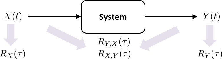
Knowing the definition of jointly WSS, we consider the cross-correlation between $X(t)$ and $Y(t)$. Note that here we are asking about the cross-correlation between the input and the output of the same LTI system, as illustrated in Figure 10.23. The pair $X(t)$ and $Y(t) = h(t)\ast X(t)$ are special because $Y(t)$ is the convolved version of $X(t)$.

**Figure 10.23.** The source of the signals when defining $R_X(\tau)$, $R_{X,Y}(\tau)$, $R_{Y,X}(\tau)$ and $R_{Y}(\tau)$.

Theorem 10.6

Let $X(t)$ and $Y(t)$ be jointly WSS processes, and let $Y(t) = h(t)\ast X(t)$. Then the cross-correlation $R_{Y,X}(\tau)$ is

R_{Y,X}(\tau)=h(\tau)\ast R_X(\tau).

Proof. Recalling the definition of cross-correlation, we have

\begin{aligned} R_{Y,X}(\tau) &= \E[Y(t+\tau)X(t)]\\ &=\E\left[X(t) \int_{-\infty}^{\infty} X(t+\tau-r)h(r)\;dr\right] \\ &=\int_{-\infty}^{\infty} \E[X(t)X(t+\tau-r)]h(r)\;dr\\ &=\int_{-\infty}^{\infty} R_X(\tau-r)h(r)\;dr, \end{aligned}

which is the convolution $R_{Y,X}(\tau)=h(\tau)\ast R_X(\tau)$.

■

We next define the cross power spectral density of two jointly WSS processes as the Fourier transform of the cross-correlation function.

Definition 10.12

The cross power spectral density of two jointly WSS processes $X(t)$ and $Y(t)$ is defined as

\begin{aligned} S_{X,Y}(\omega)&=\mathcal{F}[R_{X,Y}(\tau)], \\ S_{Y,X}(\omega)&=\mathcal{F}[R_{Y,X}(\tau)]. \end{aligned}

The relationship between $S_{X,Y}$ and $S_{Y,X}$ can be seen from the following theorem.

Theorem 10.7

For two jointly WSS random processes $X(t)$ and $Y(t)$, the cross power spectral density satisfies the property that

S_{X,Y}(\omega)= \overline{S_{Y,X}(\omega)},

where $\overline{(\cdot)}$ denotes the complex conjugate.

Proof. Since $S_{X,Y}(\omega)=\mathcal{F}[R_{X,Y}(\tau)]$ by definition, it follows that

\begin{aligned} \mathcal{F}[R_{X,Y}(\tau)] &=\int_{-\infty}^\infty R_{X,Y}(\tau) e^{-j \omega \tau} \;d\tau \\ &= \int_{-\infty}^\infty R_{Y,X}(-\tau) e^{-j \omega \tau} \;d\tau \\ &=\int_{-\infty}^\infty R_{X,Y}(\tau') e^{j \omega \tau'} \;d\tau', \end{aligned}

which is exactly the conjugate $\overline{S_{Y,X}(\omega)}$.

■

When sending the random process through an LTI system, the cross-correlation power spectral density is given by the theorem below.

Theorem 10.8

If $X(t)$ passes through an LTI system to yield $Y(t)$, then the cross power spectral density is

\begin{aligned} S_{Y,X}(\omega)&=H(\omega)S_X(\omega),\\ S_{X,Y}(\omega)&=\overline{H(\omega)}S_X(\omega). \end{aligned}

Proof. By taking the Fourier transform on $R_{Y,X}(\tau)$ we have that $S_{Y,X}(\omega)=H(\omega)S_X(\omega)$. Since $R_{X,Y}(\tau)=R_{Y,X}(-\tau)$, it holds that $S_{X,Y}(\omega)=\overline{H(\omega)}S_X(\omega)$.

■

Example 10.19

Let $X(t)$ be a WSS random process with

R_X(\tau)=e^{-\tau^2/2}, \quad H(\omega)=e^{-\omega^2/2}.

Find $S_{X,Y}(\omega)$, $R_{X,Y}(\tau)$, $S_{Y}(\omega)$ and $R_Y(\tau)$.

Solution

First, by the Fourier transform table we know that $$S_X(\omega)=\sqrt{2\pi}e^{-\omega^2/2}.$$ Since $H(\omega)=e^{-\omega^2/2}$, we have

\begin{aligned} S_{X,Y}(\omega) &= \overline{H(\omega)}S_X(\omega) =\sqrt{2\pi}e^{-\omega^2}. \end{aligned}

The cross-correlation function is

\begin{aligned} R_{X,Y}(\tau)&=\mathcal{F}^{-1}\left[\sqrt{2\pi}e^{-\omega^2}\right] =\frac{1}{\sqrt{2}} e^{-\frac{\tau^2}{4}}. \end{aligned}

The power spectral density of $Y(t)$ is

\begin{aligned} S_Y(\omega)&=|H(\omega)|^2S_X(\omega) =\sqrt{2\pi}e^{-\frac{3\omega^2}{2}}. \end{aligned}

Therefore, the autocorrelation function of $Y(t)$ is

\begin{aligned} R_Y(\tau)&=\mathcal{F}^{-1}\left[\sqrt{2\pi}e^{-\frac{3\omega^2}{2}}\right] =\frac{1}{\sqrt{3}}e^{-\tau^2/6}. \end{aligned}