eBook › Chapter 10 · Random Processes

Section 10.2

Mean and Correlation Functions

Given a random variable, we often want to know the expectation and variance, and often we also want to know the expectation and variance for the random processes. Nevertheless, we need to consider the time axis. In this section, we discuss the mean function and the autocorrelation function.

10.2.1Mean function

Definition 10.1

The mean function $\mu_X(t)$ of a random process $X(t)$ is

\mu_X(t)=\E\left[X(t)\right].

Let's consider the “expectation” of $X(t)$. Recall that a random process is actually $X(t,\xi)$ where $\xi$ is the random key. Therefore, the expectation is taken with respect to $\xi$, or to state it more explicitly,

\mu_X(t) = \E[X(t)] = \int_{\Omega} X(t,\xi)\;p(\xi)\;d\xi,

where $p(\xi)$ is the PDF of the random key. This is an abstract definition, but it is not difficult to understand if you follow the example below.

Example 10.5

Let $A\sim$Uniform$[0,1]$, and let $X(t)=A\cos(2 \pi t)$. Find $\mu_X(t)$.

Solution

The solution to this problem is actually very simple:

\begin{aligned} \mu_X(t) = \E[X(t)] &= \E[A\cos(2 \pi t)] \\ &= \cos(2 \pi t)\E[A] = \frac{1}{2} \cos(2 \pi t). \end{aligned}

So the answer is $\mu_X(t) = \frac{1}{2} \cos(2 \pi t)$.

We can link the equations to the definition more explicitly. To do so, we rewrite $X(t)$ as

X(t,\xi) = A(\xi)\cos(2\pi t).

Then we take the expectation over $A$:

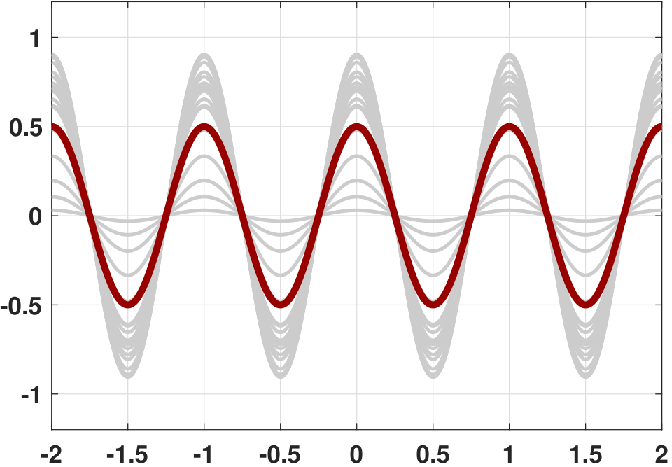
\begin{aligned} \mu_X(t) = \int_\Omega X(t,a) \;p_A(a)\; da &= \int_0^1 a \cos (2\pi t) \cdot 1 \; da \\ &= \cos(2\pi t) \bigg[\frac{a^2}{2}\bigg]_{0}^{1} = \frac{1}{2}\cos(2\pi t). \end{aligned}

An illustration is provided in Figure 10.7, in which we observe many random realizations of the random process $X(t,\xi)$. On top of these, we also see the mean function. The way to visualize the mean function is to use the statistical perspective. That is, fix a time $t$ and look at all the possible values that the function can take. For example, if we fix $t = t_0$, then we will have a set of realizations of one random variable:

\bigg\{0.71 \cos(2\pi t_0),\, 0.58\cos(2\pi t_0),\; \ldots, \; 0.93\cos(2\pi t_0)\bigg\} \; \rightarrow \; \text{take expectation}

Therefore, when we take the expectation, it is that of the underlying random variable. If we move to another timestamp $t = t_1$, we will have a different expectation because $\cos(2\pi t_0)$ now becomes $\cos(2\pi t_1)$.

The MATLAB/Python codes used to generate Figure 10.7 are shown below. You can also replace the line 0.5*cos(2*pi*t) by the mean function mean(X) (in MATLAB).

MATLAB

% MATLAB code for Example 10.5
    x = zeros(1000,20);
    t = linspace(-2,2,1000);
    for i=1:20
        X(:,i) = rand(1)*cos(2*pi*t);
    end
    plot(t, X, 'LineWidth', 2, 'Color', [0.8 0.8 0.8]); hold on;
    plot(t, 0.5*cos(2*pi*t), 'LineWidth', 4, 'Color', [0.6 0 0]);

Python

# Python code for Example 10.5
    x = np.zeros((1000,20))
    t = np.linspace(-2,2,1000)
    for i in range(20):
      x[:,i] = np.random.rand(1)*np.cos(2*np.pi*t)
    plt.plot(t,x,color='gray')
    plt.plot(t,0.5*np.cos(2*np.pi*t),color='red')
    plt.show()

Example 10.6

Let $\Theta\sim$Uniform$[-\pi,\pi]$, and let $X(t)=\cos(\omega t + \Theta)$. Find $\mu_X(t)$.

Solution

\begin{aligned} \mu_X(t) &= \E\left[\cos(\omega t + \Theta)\right] = \int_{-\pi}^\pi \cos(\omega t + \theta) \cdot \frac{1}{2\pi} \;d\theta = 0. \end{aligned}

Again, as in the previous example, we can try to map this simple calculation with the definition. Write $X(t)$ as

X(t,\xi) = \cos(\omega t + \Theta(\xi)).

Then the expectation is

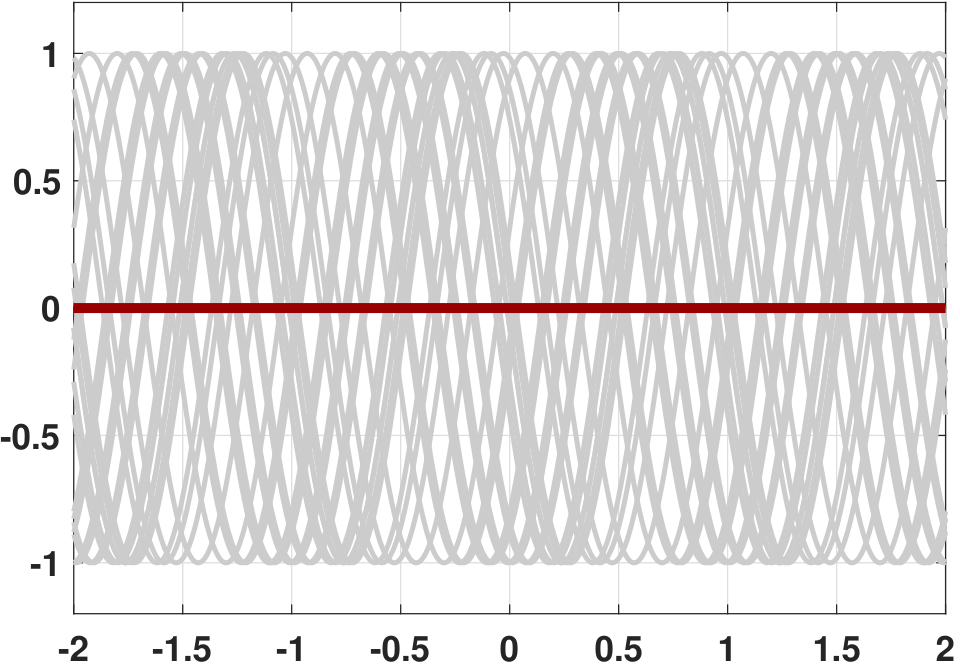
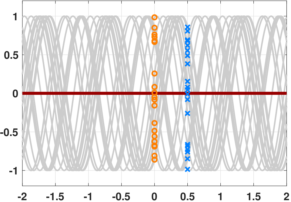
\begin{aligned} \mu_X(t) &= \int_{\Omega} \cos(\omega t + \theta) p_{\Theta}(\theta) \;d\theta\\ &= \int_{-\pi}^{\pi} \cos(\omega t + \theta) \cdot \frac{1}{2\pi} \, \;d\theta = 0. \end{aligned}

Figure 10.8 illustrates the random realizations for $X(t)=\cos(\omega t + \Theta)$ and the mean function. The zero mean should not be a surprise because if we take the statistical average (the vertical average) across all the possible values at any time instant, the positive and negative values of the realizations will make the mean zero.

We should emphasize that the statistical average is not the same as the temporal average, even if they give you the same value. Why do we say that? If we calculate the temporal average of the function $\cos(\omega t + \theta_0)$ for a specific value $\Theta = \theta_0$, then we have

\overline{X} = \frac{1}{T} \int_{0}^T \cos(\omega t + \theta_0) \;dt = 0,

assuming that $T$ is a multiple of the cosine period. This implies that the temporal average is zero, which is the same as the statistical average. This gives us an example in which the statistical average and the temporal average have the same value, although we know they are two completely different things.

The MATLAB/Python codes used to generate Figure 10.8 are shown below.

MATLAB

% MATLAB code for Example 10.6
    x = zeros(1000,20);
    t = linspace(-2,2,1000);
    for i=1:20
    X(:,i) = cos(2*pi*t+2*pi*rand(1));
    end
    plot(t, X, 'LineWidth', 2, 'Color', [0.8 0.8 0.8]); hold on;
    plot(t, 0*cos(2*pi*t), 'LineWidth', 4, 'Color', [0.6 0 0]);

Python

# Python code for Example 10.6
    x = np.zeros((1000,20))
    t = np.linspace(-2,2,1000)
    for i in range(20):
      Theta = 2*np.pi*(np.random.rand(1))
      x[:,i] = np.cos(2*np.pi*t+Theta)
    plt.plot(t,x,color='gray')
    plt.plot(t,np.zeros((1000,1)),color='red')
    plt.show()

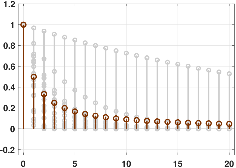
Example 10.7

Let us consider a discrete-time random process. Let $X[n]=S^n$, where $S\sim$Uniform$[0,1]$. Find $\mu_X[n]$.

\begin{aligned} \mu_X[n] &= \E[s^n] = \int_0^1 s^n \;ds = \frac{1}{n+1}. \end{aligned}

In this example the randomness goes with the constant $s$. Thus, if we write $X[n]$ as

\begin{aligned} X[n,\xi] = [S(\xi)]^n, \end{aligned}

the expectation is

\begin{aligned} \E[X[n]] = \int_{\Omega} s^n p_S(s) \;ds = \int_{0}^1 s^n \cdot 1 \;ds = \frac{1}{n+1}. \end{aligned}

The graphical illustration is provided in Figure 10.9.

The MATLAB code used to generate Figure 10.9 is shown below. We skip the Python implementation because it is straightforward.

MATLAB

% MATLAB code for Example 10.7
    t = 0:20;
    for i=1:20
        X(:,i) = rand(1).^t;
    end
    stem(t, X, 'LineWidth', 2, 'Color', [0.8 0.8 0.8]); hold on;
    stem(t, 1./(t+1), 'LineWidth', 2, 'MarkerSize', 8);

10.2.2Autocorrelation function

In random processes, the notions of “variance” and “covariance” are trickier than for random variables. Let us first define the concept of an autocorrelation function.

Definition 10.2

The autocorrelation function of a random process $X(t)$ is

R_{X}(t_1,t_2)=\E\left[X(t_1)X(t_2)\right].

$R_{X}(t_1,t_2)$ is not difficult to calculate — just integrate $X(t_1)X(t_2)$ using the appropriate PDFs.

Example 10.8

Let $A\sim$Uniform$[0,1]$, $X(t)=A\cos(2\pi t)$. Find $R_X(t_1,t_2)$.

Solution

\begin{aligned} R_X(t_1,t_2) &= \E\left[A\cos(2\pi t_1)A\cos(2\pi t_2)\right] \\ &= \E[A^2]\cos(2\pi t_1)\cos(2\pi t_2) = \frac{1}{3}\cos(2\pi t_1)\cos(2\pi t_2). \end{aligned}

Example 10.9

Let $\Theta\sim$Uniform$[-\pi,\pi]$, $X(t)=\cos(\omega t + \Theta)$. Find $R_X(t_1,t_2)$.

Solution

\begin{aligned} R_X(t_1,t_2) &= \E\left[\cos(\omega t_1 + \Theta)\cos(\omega t_2 + \Theta)\right] \\ &= \frac{1}{2\pi}\int_{-\pi}^{\pi} \cos(\omega t_1 + \theta)\cos(\omega t_2 + \theta) \;d\theta\\ &\overset{(a)}{=} \frac{1}{2\pi}\int_{-\pi}^{\pi} \frac{1}{2}\bigg[\cos(\omega(t_1+t_2) + 2\theta) + \cos(\omega (t_1-t_2) )\bigg] \;d\theta\\ &= \frac{1}{2} \cos\Big(\omega(t_1-t_2)\Big), \end{aligned}

where in (a) we applied the trigonometric formula $\cos A \cos B = \frac{1}{2}[\cos(A+B) + \cos (A-B)]$.

As you can see, the calculations are not difficult. The tricky thing is the interpretation of $R_X(t_1,t_2)$.

How do we understand the meaning of $\E[X(t_1)X(t_2)]$?

$\E\left[X(t_1)X(t_2)\right]$ is analogous to the correlation $\E[XY]$ between $X$ and $Y$.

The autocorrelation function $\E\left[X(t_1)X(t_2)\right]$ is analogous to the correlation $\E[XY]$ in relation to a pair of random variables. In our discussions of $\E[XY]$, we mentioned that $\E[XY]$ could be regarded as the inner product of two vectors, and so it is a measure of the closeness between $X$ and $Y$. Now, if we substitute $X$ and $Y$ with $X(t_1)$ and $X(t_2)$ respectively, then we are effectively asking about the closeness between $X(t_1)$ and $X(t_2)$. So, in a nutshell, the autocorrelation function tells us the correlation between the function at two different time stamps.

What do we mean by the correlation between two timestamps? Remember that $X(t_1)$ and $X(t_2)$ are two random variables. Consider the following example.

Example 10.10

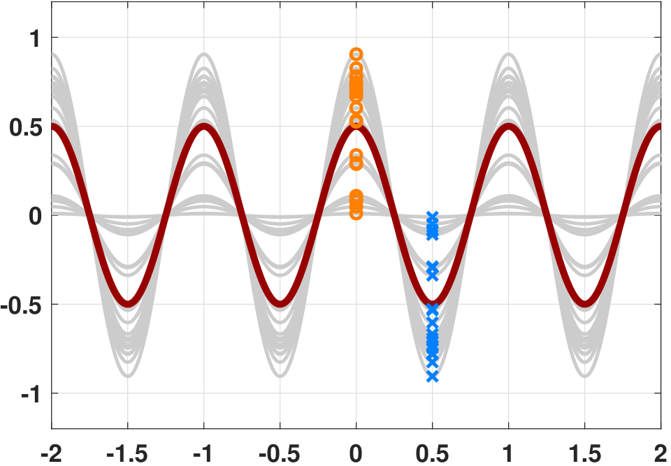
Let $X(t) = A\cos(2\pi t)$, where $A \sim \text{Uniform}[0,1]$. Find $\E[X(0)X(0.5)]$.

Solution

If $X(t) = A\cos(2\pi t)$, then

\begin{aligned} X(0) &= A\cos(0) = A,\\ X(0.5) &= A\cos(\pi) = -A. \end{aligned}

When you have two random variables, you consider their correlations. Using this example, we have that

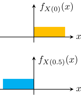
\begin{aligned} \E[X(0)X(0.5)] &= -\E[A\cdot A] = -\E[A^2] = -\frac{1}{3}. \end{aligned}

A picture will reveal what is happening. Figure 10.10 presents the realizations of the random process $X(t) = A\cos(2\pi t)$. If we consider $X(0)$ and $X(0.5)$, each of them is a random variable, and thus we can ask about their PDFs. It is obvious from the illustration that the random variable $X(0)$ has a PDF that is a uniform distribution from 0 to 1, whereas the random variable $X(0.5)$ has a PDF that is a uniform distribution from $-1$ to $0$. Mathematically, the PDFs are

f_{X(0)}(x) = \begin{cases} 1, \quad 0 \le x \le 1,\\ 0, \quad \text{otherwise} \end{cases} \qquad\text{and}\qquad f_{X(0.5)}(x) = \begin{cases} 1, \quad -1 \le x \le 0,\\ 0, \quad \text{otherwise}. \end{cases}

Since $X(0)$ and $X(0.5)$ have their own PDFs, we can calculate their correlation. This will give us $\E[X(0)X(0.5)]$ which after some calculations is $\E[X(0)X(0.5)] = -\frac{1}{3}$.

We can now consider the autocorrelation for any $t_1$ and $t_2$. When you are evaluating the autocorrelation function, you are not just evaluating at $t = 0$ and $t = 0.5$, you are also evaluating the correlation for all pairs of $t_1$ and $t_2$. Now you want to know what the correlation is between $t = 0$ and $t = 0.5$, $t = 2$ and $t = 3.1$, etc. Of course, there are infinitely many pairs of time instants. The point of the autocorrelation function is to tell you the correlation of all the pairs. In other words, if we tell you $R_X(t_1,t_2)$, you will be able to plug in a value of $t_1$ and a value of $t_2$ and tell us the correlation at $(t_1,t_2)$. How is this possible? To find out, let's consider the following example.

Example 10.11

Let $A\sim$Uniform$[0,1]$, $X(t)=A\cos(2\pi t)$. Find $R_X(0,0.5)$, and draw $R_X(t_1,t_2)$.

Solution

From the previous example, we know that

\begin{aligned} R_X(t_1,t_2)= \frac{1}{3}\cos(2\pi t_1)\cos(2\pi t_2). \end{aligned}

Therefore, $R_X(0,0.5) = \frac{1}{3}\cos(2\pi 0)\cos(2\pi 0.5) = -\frac{1}{3}$, which is the same as if we had computed it from first principles.

The autocorrelation function tells you how one point of a time series is correlated with another point of the time series. If $R_X(t_1,t_2)$ gives a high value, then it means the random variables at $t_1$ and $t_2$ have a strong correlation. To understand this, suppose we let $t_1 = 0$, and let us vary $t_2$. Then

\begin{aligned} R_X(0,t_2) &= \frac{1}{3}\cos(2\pi 0)\cos(2\pi t_2) \\ &= \frac{1}{3} \cos(2\pi t_2). \end{aligned}

This is a periodic function that cycles through itself whenever $t_2$ is an integer. As we recall from Figure 10.10, if $t_2 = 0.5$, the random variable $X(t_2)$ will take only the negative values, but otherwise it is correlated with $X(0)$. On the other hand, if $t_2 = 0.25$, then Figure 10.10 says that the random variable $X(t_2)$ is a constant 0, and so the correlation with $X(0)$ is zero.

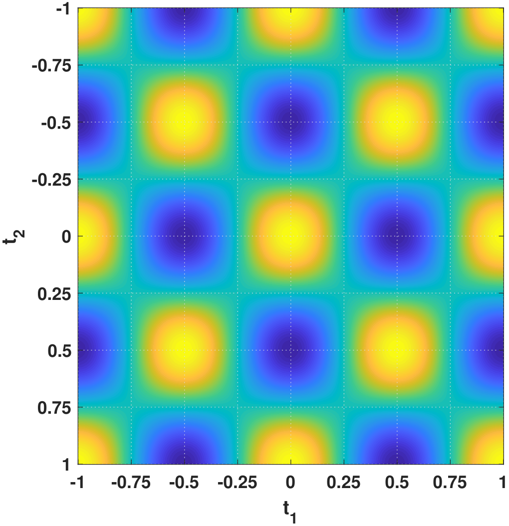
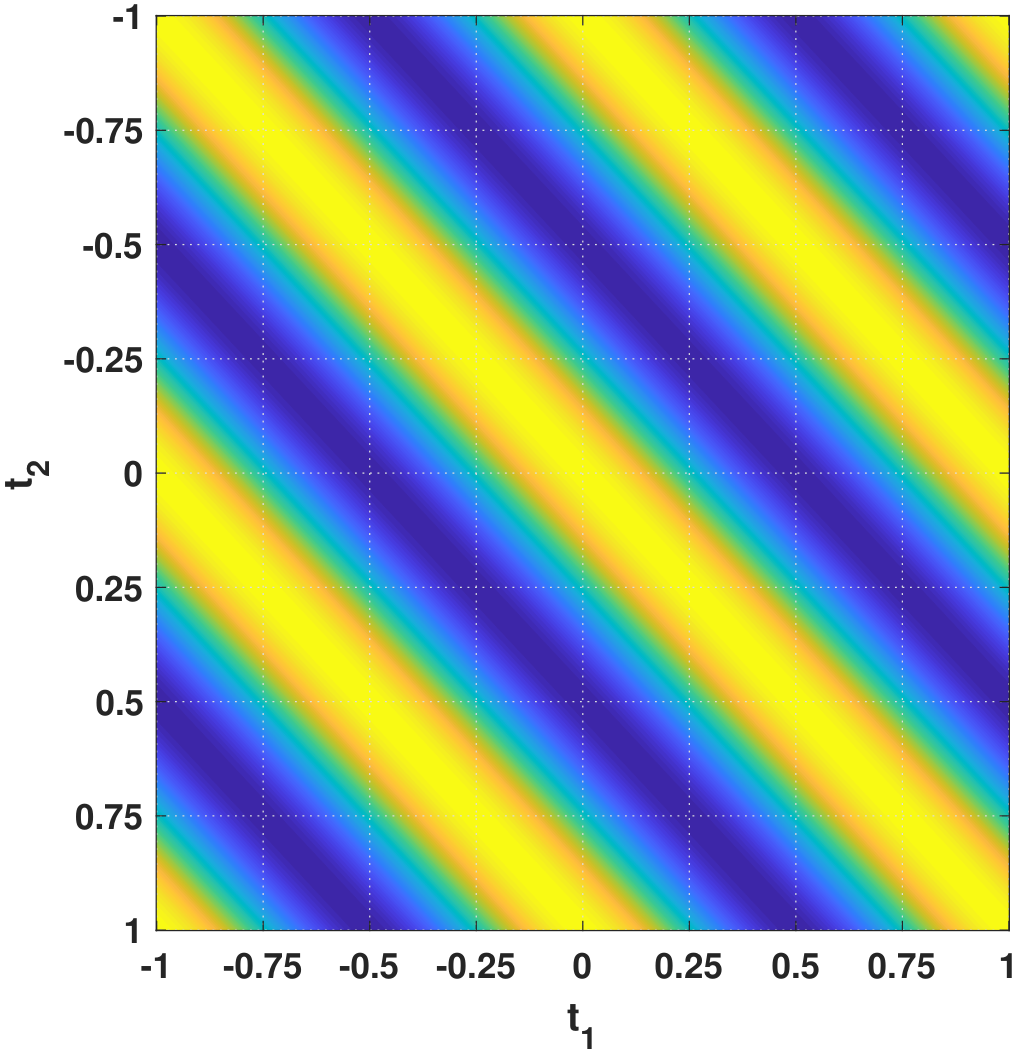
**Figure 10.10.** The autocorrelation between $X(0)$ and $X(0.5)$ should be regarded as the correlation between two random variables. Each random variable has its own PDF.

Clearly, $R_X(t_1,t_2)$ is a 2-dimensional function of $t_1$ and $t_2$. You need to tell $R_X$ which of the two time instants you want to compare, and then $R_X$ will tell you the correlation. So no matter what happens, you must specify two time instants. Because $R_X(t_1,t_2)$ is a 2-dimensional function, we can visualize it by calculating all the possible values it takes. For example, if $R_X(t_1,t_2) = \frac{1}{3}\cos(2\pi t_1)\cos(2\pi t_2)$, we can plot $R_X$ as a function of $t_1$ and $t_2$. Figure 10.11 shows the plot.

**Figure 10.11.** The autocorrelation function $R_X(t_1,t_2) = \frac{1}{3}\cos(2\pi t_1)\cos(2\pi t_2)$.

The MATLAB/Python code for Figure 10.11 is shown below.

MATLAB

% MATLAB code for Example 10.11
    t = linspace(-1,1,1000);
    R = (1/3)*cos(2*pi*t(:)).*cos(2*pi*t);
    imagesc(t,t,R);

Python

# Python code for Example 10.11
    import numpy as np
    import matplotlib.pyplot as plt
    t = np.linspace(-1,1,1000)
    R = (1/3)*np.outer(np.cos(2*np.pi*t), np.cos(2*np.pi*t))
    plt.imshow(R, extent=[-1, 1, -1, 1])
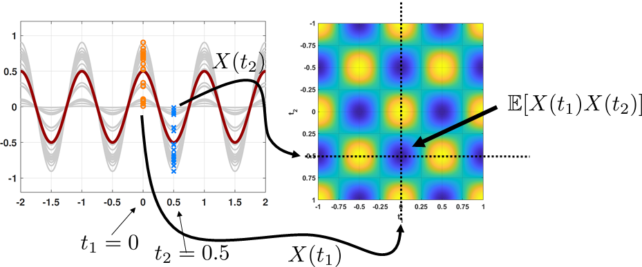
    plt.show()

To understand the 2D function shown on the right-hand side of Figure 10.11, we can take a closer look by drawing Figure 10.12. For any two time instants $t_1$ and $t_2$, we have two random variables $X(t_1)$ and $X(t_2)$. The joint expectation $\E[X(t_1)X(t_2)]$ will return us some value, and this is a point in the 2D plot $R_{X}(t_1,t_2)$. The value tells us the correlation between $X(t_1)$ and $X(t_2)$. In the example in which $t_1 = 0$ and $t_2 = 0.5$, the correlation is $-\frac{1}{3}$. Interestingly, if we pick another pair of time instants $t_1 = -0.5$ and $t_2 = 0$, the joint expectation is $\E[X(-0.5)X(0)] = -\frac{1}{3}$, which is the same value. However, this $-\frac{1}{3}$ is located at a different valley than $\E[X(0)X(0.5)]$ in the 2D plot.

The above example shows a periodic autocorrelation function. The fact that it is periodic is coincidental because the random process $X(t)$ is a periodic function. In general, an arbitrary random process can have an arbitrary autocorrelation function that is not periodic. There are, of course, various properties of the autocorrelation functions and special types of autocorrelation functions. We will study one of them, called the wide-sense stationary processes, later.

Example 10.12

Let $\Theta\sim$Uniform$[-\pi,\pi]$, $X(t)=\cos(\omega t + \Theta)$. Draw the autocorrelation function $R_X(t_1,t_2)$.

Solution

From the previous example we know that

\begin{aligned} R_X(t_1,t_2) = \frac{1}{2} \cos\Big(\omega(t_1-t_2)\Big). \end{aligned}

Figure 10.13 shows the realizations, and the mean and autocorrelation functions.

Note that the autocorrelation function has a structure: Every row is a shifted version of the previous row. We call this a Toeplitz structure. An autocorrelation with a Toeplitz structure is specified once we know any of the rows. A Toeplitz structure also implies that the autocorrelation function does not depend on the pair $(t_1,t_2)$ but only on the difference $t_1-t_2$. In other words, $R_X(0,1)$ is the same as $R_X(11.6,12.6)$, and so knowing $R_X(0,1)$ is enough to know all $R_X(t_0,t_0+t)$. Not all random processes have a Toeplitz autocorrelation function. Random processes with a Toeplitz autocorrelation function are “nice” processes that we will study in detail later.

**Figure 10.13.** The autocorrelation function $R_X(t_1,t_2) = \frac{1}{2} \cos\Big(\omega(t_1-t_2)\Big)$.

The MATLAB code used to generate Figure 10.13 is shown below.

MATLAB

% MATLAB code for Example 10.12
    t = linspace(-1,1,1000);
    R = Toeplitz(0.5*cos(2*pi*t(:)));
    
    imagesc(t,t,R);
    grid on;
    xticks(-1:0.25:1);
    yticks(-1:0.25:1);

Practice Exercise 10.1

Let $\Theta\sim$Uniform$[0,2\pi]$, $X(t)=\cos(\omega t + \Theta)$. Find the PDF of $X(0)$.

Solution

Let $Z = X(0) = \cos \Theta$. Then the CDF of $Z$ is

\begin{aligned} F_Z(z) &= \Pb[Z \le z] \\ &= \Pb[\cos\Theta \le z] \\ &= \Pb[\cos^{-1}z \le \Theta \le 2\pi - \cos^{-1}z] \\ &= 1- \frac{\cos^{-1}z}{\pi}. \end{aligned}

Then by the fundamental theorem of calculus, $$f_Z(z) = \frac{1}{\pi\sqrt{1-z^2}}.$$

A similar concept to the autocorrelation function is the autocovariance function. The idea is to remove the mean before computing the correlation. This is analogous to the covariance $\Cov(X,Y) = \E[(X-\mu_X)(Y-\mu_Y)]$ as opposed to the correlation $\E[XY]$ in the random variable case.

Definition 10.3

The autocovariance function of a random process $X(t)$ is

C_{X}(t_1,t_2)=\E\left[\left(X(t_1)-\mu_X(t_1)\right)\left(X(t_2)-\mu_X(t_2)\right)\right].

As one might expect, the autocovariance function is closely related to the autocorrelation function.

Theorem 10.1

C_{X}(t_1,t_2)=R_{X}(t_1,t_2)-\mu_X(t_1)\mu_X(t_2).

Proof. Plugging in the definition, we have that

\begin{aligned} C_{X}(t_1,t_2) %&= \E\left[\left(X(t_1)-\mu_X(t_1)\right)\left(X(t_2)-\mu_X(t_2)\right)\right]\\ &= \E\left[X(t_1)X(t_2)-X(t_1)\mu_X(t_2)-X(t_2)\mu_X(t_1)+\mu_X(t_1)\mu_X(t_2)\right] \\ &= R_{X}(t_1,t_2)-\mu_X(t_1)\mu_X(t_2)-\mu_X(t_1)\mu_X(t_2)+\mu_X(t_1)\mu_X(t_2) \\ &= R_{X}(t_1,t_2)-\mu_X(t_1)\mu_X(t_2). \end{aligned}

■

Practice Exercise 10.2

If $X(t) = A\cos(2\pi t)$ for $A \sim \text{Uniform}[0,1]$, find $C_X(t_1,t_2)$.

Solution

\begin{aligned} C_X(t_1,t_2) %&= R_X(t_1,t_2) - \mu_X(t_1)\mu_X(t_2) \\ &= \frac{1}{3}\cos(2\pi t_1)\cos(2\pi t_2) - \frac{1}{2}\cos(2\pi t_1) \cdot \frac{1}{2}\cos(2\pi t_2) \\ &= \frac{1}{12}\cos(2\pi t_1)\cos(2\pi t_2). \end{aligned}

Practice Exercise 10.3

Suppose $X(t) = \cos(\omega t + \Theta)$ for $\Theta \sim \text{Uniform}[-\pi,\pi]$. Find $C_X(t_1,t_2)$.

Solution

\begin{aligned} C_X(t_1,t_2) &= R_X(t_1,t_2) - \mu_X(t_1)\mu_X(t_2) \\ &= \frac{1}{2}\cos\bigg(\omega(t_1-t_2)\bigg) - 0\cdot 0 = \frac{1}{2}\cos\bigg(\omega(t_1-t_2)\bigg). \end{aligned}

In some problems we are interested in the correlation between two random processes $X(t)$ and $Y(t)$. This gives us the cross-correlation and the cross-covariance functions.

Definition 10.4

The cross-correlation function of $X(t)$ and $Y(t)$ is

R_{X,Y}(t_1,t_2)=\E\left[X(t_1)Y(t_2)\right].

Definition 10.5

The cross-covariance function of $X(t)$ and $Y(t)$ is

C_{X,Y}(t_1,t_2)=\E\left[\left(X(t_1)-\mu_X(t_1)\right)\left(Y(t_2)-\mu_Y(t_2)\right)\right].

Remark. If $\mu_X(t_1) = \mu_Y(t_2) = 0$, then $C_{X,Y}(t_1,t_2)=R_{X,Y}(t_1,t_2)=\E[X(t_1)Y(t_2)]$.

10.2.3Independent processes

How do we establish independence for two random processes? We know that for two random variables to be independent, the joint PDF can be written as a product of two PDFs:

f_{X,Y}(x,y) = f_X(x)f_Y(y).

If we extrapolate this idea to random processes, a natural formulation would be

f_{X(t),Y(t)}(x,y) = f_{X(t)}(x)f_{Y(t)}(y).

But this definition has a problem because $X(t)$ and $Y(t)$ are functions. It is not enough to just look at one time index, say $t = t_0$. The way to think about this situation is to consider a pair of random vectors $\mX$ and $\mY$. When you say $\mX$ and $\mY$ are independent, you require $f_{\mX,\mY}(\vx,\vy) = f_{\mX}(\vx)f_{\mY}(\vy)$. The PDF $f_{\mX}(\vx)$ itself is a joint distribution, i.e., $f_{\mX}(\vx) = f_{X_1,\ldots,X_N}(x_1,\ldots,x_N)$. Therefore, for random processes, we need something similar.

Definition 10.6

Two random processes $X(t)$ and $Y(t)$ are independent if for any $t_1,\ldots,t_N$,

\begin{aligned} &f_{X(t_1),\ldots,X(t_N),Y(t_1),\ldots,Y(t_N)}(x_1,\ldots,x_N,y_1,\ldots,y_N) \\ &\qquad\qquad= f_{X(t_1),\ldots,X(t_N)}(x_1,\ldots,x_N) \times f_{Y(t_1),\ldots,Y(t_N)}(y_1,\ldots,y_N). \end{aligned}

This definition is reminiscent of $f_{\mX,\mY}(\vx,\vy) = f_{\mX}(\vx)f_{\mY}(\vy)$. The requirement here is that the factorization holds for any $N$, including very small $N$ and very large $N$, because $X(t)$ and $Y(t)$ are infinitely long.

Independence means that the behavior of one process will not influence the behavior of the other process. We define uncorrelated as follows.

Definition 10.7

Two random processes $X(t)$ and $Y(t)$ are uncorrelated if

\E\left[X(t_1)Y(t_2)\right] = \E\left[X(t_1)\right]\E\left[Y(t_2)\right],

Independence implies uncorrelation, as we can see from the following. If $X(t)$ and $Y(t)$ are independent, it follows that

\begin{aligned} \E\left[X(t_1)Y(t_2)\right] &= \int X(t_1,\xi)Y(t_2,\zeta) f_{X,Y}(\xi,\zeta) \;d\xi \;d\zeta \\ &= \int X(t_1,\xi) Y(t_2,\zeta) f_X(\xi) f_Y(\zeta) \;d\xi \;d\zeta, \qquad \text{independence}\\ &= \int X(t_1,\xi) f_X(\xi) \; d\xi \int Y(t_2,\zeta) f_Y(\zeta) \;d\zeta = \E[X(t_1)]\E[Y(t_2)]. \end{aligned}

If two random processes are uncorrelated, they are not necessarily independent.

$$\textrm{Independent X and Y} \begin{array}{c} \Rightarrow \\ \nLeftarrow \end{array} \textrm{uncorrelated X and Y}$$

Example 10.13

Let $Y(t)=X(t)+N(t)$, where $X(t)$ and $N(t)$ are independent. Then

\begin{aligned} R_{X,Y}(t_1,t_2) = \E\left[X(t_1)Y(t_2)\right] &= \E\left[X(t_1)\left(X(t_2)+N(t_2)\right)\right] \\ &= R_{X}(t_1,t_2)+\mu_X(t_1)\mu_N(t_2). \end{aligned}