eBook › Chapter 10 · Random Processes

Section 10.6

Optimal Linear Filter

In the previous sections, we have built many tools to analyze random processes. Our next goal is to apply these techniques. To that end, we will discuss optimal linear filter design, which is a set of estimation techniques for predicting and recovering information from a time series.

10.6.1Discrete-time random processes

We begin by introducing some notations. In the previous sections, we have been using continuous-time random processes to study statistics. In this section, we mainly focus on discrete-time random processes. The shift from continuous-time to discrete-time is straightforward as far as the theories are concerned — we switch the continuous-time index $t$ to a discrete-time index $n$. However, shifting to discrete-time random processes can simplify many difficult problems because many discrete-time problems can be solved by matrices and vectors. This will make the computations and implementations much easier. To make this transition easier, we provide a few definitions and results without proof.

Notations for discrete-time random processes

sep0ex
We denote the discrete-time indices by $m$ and $n$, corresponding to the continuous-time indices $t_1$ and $t_2$, respectively.
A discrete-time random process is denoted by $X[n]$.
Its mean function and the autocorrelation function are
$\begin{aligned} \mu_X[n] &= \E[X[n]],\\ R_X[m,n] &= \E[X[m]X[n]]. \end{aligned}$
We say that $X[n]$ is WSS if $\mu_X[n] =$ constant, and $R_X[m,n]$ is a function of $m-n$.
If $X[n]$ is WSS, we write $R_X[m,n]$ as
$$$R_X[m,n] = R_X[m-n] = R_X[k],$$$
where $k = m-n$ is the interval.
If $X[n]$ is WSS, we define the power spectral density as
$S_X(e^{j\omega}) = \calF\{R_X[k]\},$
where $S_X(e^{j\omega})$ denotes the discrete-time Fourier transform.

When a random process $X[n]$ is sent through an LTI system with an impulse response $h[n]$, the output is

Y[n] = h[n] \ast X[n] = \sum_{k=-\infty}^{\infty} h[k] X[n-k].

When a WSS process $X[n]$ passes through an LTI system $h[n]$ to yield an output $Y[n]$, the auto- and cross-correlation function and power spectral densities are

sep0ex
$R_Y[k] = \E[Y[n+k]Y[n]]$, $S_Y(e^{j\omega}) = \calF\{R_Y[k]\} = |H(e^{j\omega})|^2S_X(e^{j\omega})$.
$R_{XY}[k] = \E[X[n+k]Y[n]]$, $S_{XY}(e^{j\omega}) = \calF\{R_{XY}[k]\} = \overline{H(e^{j\omega})}S_X(e^{j\omega})$.
$R_{YX}[k] = \E[Y[n+k]X[n]]$, $S_{YX}(e^{j\omega}) = \calF\{R_{YX}[k]\} = H(e^{j\omega})S_X(e^{j\omega})$.

10.6.2Problem formulation

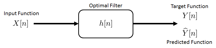
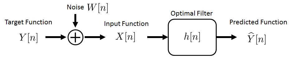
The problem we study here is known as the optimal linear filter design. Suppose that there is a WSS process $X[n]$ that we want to process. For example, if $X[n]$ is a corrupted version of some clean time-series, we may want to remove the noise by filtering (also known as averaging) $X[n]$. Conceptualizing the denoising process as a linear time-invariant system with an impulse response $h[n]$, our goal is to determine the optimal $h[n]$ such that the estimated time series $\widehat{Y}[n]$ is as close to the true time series $Y[n]$ as possible.

Referring to Figure 10.24, we refer to $X[n]$ as the input function and to $Y[n]$ as the target function. $X[n]$ and $Y[n]$ are related according to the equation

Y[n] = \underset{\widehat{Y}[n]}{\underbrace{\sum_{k=0}^{K-1} h[k]X[n-k]}} + E[n],

where $E[n]$ is a noise random process to model the error. The linear part of the equation is known as the prediction and is constructed by sending $X[n]$ through the system. For simplicity we assume that $X[n]$ is WSS. Thus, it follows that $Y[n]$ is also WSS. We may also assume that we can estimate $R_X[k]$, $R_{YX}[k]$, $R_{XY}[k]$ and $R_{Y}[k]$.

**Figure 10.24.** A schematic diagram illustrating the optimal linear filter problem: Given an input function $X[n]$, we want to design a filter $h[n]$ such that the prediction $\widehat{Y}[n]$ is close to the target function $Y[n]$.

Example 10.20

If we let $K = 3$, Eq. (10.34) gives us

\begin{aligned} Y[n] = h[0]X[n] + h[1]X[n-1] + h[2]X[n-2] + E[n]. \end{aligned}

That is, the current sample $Y[n]$ is a linear combination of the previous samples $X[n]$, $X[n-1]$ and $X[n-2]$.

Given $X[n]$ and $Y[n]$, what would be the best guess of the impulse response $h[n]$ so that the prediction is as close to the true values as possible? From our discussions of linear regression, we know that this is equivalent to solving the optimization problem

\begin{aligned} \minimize{\{h[k]\}_{k=0}^{K-1}} \;\; \left( Y[n] - \sum_{k=0}^{K-1} h[k]X[n-k] \right)^2. \end{aligned}

The choice of the squared error is more or less arbitrary, depending on how we want to model $E[n]$. By using the squared norm, we implicitly assume that the error is Gaussian. This may not be true, but it is commonly used because the squared norm is differentiable. We will follow this tradition.

The challenge associated with the minimization is that in most of the practical settings the random processes $X[n]$ and $Y[n]$ are changing rapidly because they are random processes. Therefore, even if we solve the optimization problem, the estimates $h[k]$ will be random variables since we are solving a random equation. To eliminate this randomness, we take the expectation over all the possible choices of $X[n]$ and $Y[n]$, yielding

\begin{aligned} \minimize{\{h[k]\}_{k=0}^{K-1}} &\; \qquad\quad \left( Y[n] - \sum_{k=0}^{K-1} h[k]X[n-k] \right)^2,\\ &\qquad\qquad\qquad\qquad\Downarrow \\ \minimize{\{h[k]\}_{k=0}^{K-1}} &\;\; \textcolor{blue}{\E_{X,Y}} \left[ \left( Y[n] - \sum_{k=0}^{K-1} h[k]X[n-k] \right)^2\right]. \end{aligned}

The resulting impulse response $h[k]$, derived by solving the above minimization, is known as the optimal linear filter. It is the best linear model for describing the input-output relationships between $X[n]$ and $Y[n]$.

What is the optimal linear filter?

The optimal linear filter is the solution to the optimization problem

\minimize{\{h[k]\}_{k=0}^{K-1}} \;\; \E_{X,Y} \left[\left( Y[n] - \sum_{k=0}^{K-1} h[k]X[n-k] \right)^2\right].

10.6.3Yule-Walker equation

To solve the optimal linear filter problem, we first perform some (slightly tedious) algebra to obtain the following results:

Lemma 10.4

Let $\widehat{Y}[n] = \sum_{k=0}^{K-1} h[k]X[n-k]$ be the prediction of $Y[n]$. The squared-norm error can be written as

\begin{aligned} &\E_{X,Y}\left[\left( Y[n] - \widehat{Y}[n] \right)^2\right] \\ &= R_Y[0] - 2 \sum_{k=0}^{K-1} h[k] R_{YX}[k] + \sum_{k=0}^{K-1} \sum_{j=0}^{K-1} h[k] h[j] R_{X}[j-k]. \end{aligned}

Thus we can express the error in terms of $R_{YX}[k]$, $R_X[k]$ and $R_Y[k]$.

Proof. We expand the error as follows:

\begin{aligned} \E_{X,Y}\left[\left( Y[n] - \widehat{Y}[n] \right)^2\right] = \E_{Y}\left[ (Y[n])^2 \right] -2 \E_{X,Y}\left[ Y[n]\widehat{Y}[n] \right] + \E_{X}\left[ (\widehat{Y}[n])^2 \right]. \end{aligned}

The first term is the autocorrelation of $Y[n]$:

\begin{aligned} \E_{Y}\left[ (Y[n])^2 \right] &= \E\left[ Y[n+0]Y[n] \right] = R_Y[0]. \end{aligned}

The second term is

\begin{aligned} \E_{X,Y}\left[ Y[n]\widehat{Y}[n] \right] &= \E_{X,Y}\left[ Y[n] \sum_{k=0}^{K-1} h[k]X[n-k] \right] \\ &= \sum_{k=0}^{K-1} h[k] \E_{X,Y}\left[ Y[n] X[n-k] \right] \\ &= \sum_{k=0}^{K-1} h[k] R_{YX}[k]. \end{aligned}

The third term is

\begin{aligned} \E_{X}\left[ (\widehat{Y}[n])^2 \right] &= \E_{X}\left[ \left(\sum_{k=0}^{K-1} h[k] X[n-k] \right)\left( \sum_{j=0}^{K-1} h[j] X[n-j] \right) \right]\\ &= \E_{X}\left[ \sum_{k=0}^{K-1} \sum_{j=0}^{K-1} h[k] h[j] X[n-k] X[n-j] \right]\\ &= \sum_{k=0}^{K-1} \sum_{j=0}^{K-1} h[k] h[j] \E_{X}\left[ X[n-k] X[n-j] \right]\\ &= \sum_{k=0}^{K-1} \sum_{j=0}^{K-1} h[k] h[j] R_{X}[j-k]. \end{aligned}

This completes the proof.

■

The significance of this theorem is that it allows us to write the error in terms of $R_{YX}[k]$, $R_X[k]$ and $R_Y[k]$. As we have mentioned, while we can solve the randomized optimization Eq. (10.35), the resulting solution will be a random vector depending on the particular realizations $X[n]$ and $Y[n]$. Switching from Eq. (10.35) to Eq. (10.36) eliminates the randomness because we have taken the expectation. The resulting optimization according to the theorem is also convenient. Instead of seeking individual realizations, we only need to know the overall statistical description of the data through $R_{YX}[k]$, $R_X[k]$ and $R_Y[k]$. These can be estimated through modeling or pseudorandom signals.

The solution to the optimal linear filter problem is summarized by the Yule-Walker equation:

Theorem 10.9

The solution $\{h[0],\ldots,h[K-1]\}$ to the optimal linear filter problem

\minimize{\{h[k]\}_{k=0}^{K-1}} \;\; \E_{X,Y} \left[\left( Y[n] - \sum_{k=0}^{K-1} h[k]X[n-k] \right)^2\right]

is given by the following matrix equation:

\left( \begin{array}{c} R_{YX}[0] \\ R_{YX}[1] \\ \vdots \\ R_{YX}[K-1] \\ \end{array} \right)=\left( \begin{array}{cccc} R_X[0] & R_X[1] & \cdots & R_X[K-1] \\ R_X[1] & R_X[0] & \cdots & \vdots \\ \vdots & \vdots & \ddots & \vdots \\ R_X[K-1] & R_X[K-2] & \cdots & R_X[0] \\ \end{array} \right)\left( \begin{array}{c} h[0] \\ h[1] \\ \vdots \\ h[K-1] \\ \end{array} \right),

which is known as the Yule-Walker equation.

Therefore, by solving the simple linear problem given by the Yule-Walker equation, we will find the optimal linear filter solution.

Proof. Since the error is a squared norm, the optimal solution is obtained by taking the derivative:

\begin{aligned} &\frac{d}{dh[i]} \E_{X,Y}\left[\left( Y[n] - \widehat{Y}[n] \right)^2\right]\\ &= \frac{d}{dh[i]} \left\{R_Y[0] -2 \sum_{k=0}^{K-1} h[k] R_{YX}[k] + \sum_{k=0}^{K-1} \sum_{j=0}^{K-1} h[k] h[j] R_{X}[j-k]\right\}\\ &=0 - 2 R_{YX}[i] + 2 \sum_{k=0}^{K-1} h[k] R_X[i-k], \end{aligned}

in which the derivative of the last term is computed by noting that

\begin{aligned} &\frac{d}{dh[i]}\sum_{k=0}^{K-1} \sum_{j=0}^{K-1} h[k] h[j] R_{X}[j-k]\\ &= \frac{d}{dh[i]} \sum_{j=0}^{K-1} h[j]^2 R_X[0] + \frac{d}{dh[i]} \sum_{k=0}^{K-1} \sum_{j\not=k} h[k] h[j] R_{X}[j-k]\\ &= 2 \sum_{k=0}^{K-1} h[k] R_X[i-k]. \end{aligned}

Equating the derivative to zero yields

R_{YX}[i] = \sum_{k=0}^{K-1} h[k] R_X[i-k], \qquad i = 0,\ldots,K-1,

and putting the above equations into the matrix-vector form we complete the proof.

■

The matrix in the Yule-Walker equation is a Toeplitz matrix, in which each row is a shifted version of the preceding row. This matrix structure is a consequence of a WSS process so that the autocorrelation function is determined by the time difference $k$ and not by the starting and end times.

Remark. If we take the derivative of the loss w.r.t. $h[i]$, we have that

\begin{aligned} 0 &=\frac{d}{dh[i]} \E_{X,Y}\left[\left( Y[n] - \widehat{Y}[n] \right)^2\right] = -2 \E\left[ \left(Y[n] - \widehat{Y}[n]\right) X[n-i] \right]. \end{aligned}

This condition is known as the orthogonality condition, as it says that the error $Y[n]-\widehat{Y}[n]$ is orthogonal to the signal $X[n-i]$.

10.6.4Linear prediction

We now demonstrate how to use the Yule-Walker equation in modeling an autoregressive process. The procedure in this simple example can be used in speech processing and time-series forecasting.

Suppose that we have a WSS random process $Y[n]$. We would like to predict the future samples by using the most recent $K$ samples through an autoregressive model. Since the model is linear, we can write

\begin{aligned} Y[n] = \sum_{k=1}^K h[k] Y[n-k] + E[n]. \end{aligned}

In this model, we say that the predicted value $\widehat{Y}[n]$ is a linear combination of the past $K$ samples, albeit with an approximation error $E[n]$.

The problem we need to solve is

\begin{aligned} \minimize{h[k]} \;\; \E\left[\left(Y[n] - \widehat{Y}[n]\right)^2\right]. \end{aligned}

Since $\widehat{Y}[n]$ is written in terms of the past samples of $Y[n]$ in this problem, in the Yule-Walker equation we can replace $X$ with $Y$. Consequently, we can write the matrix equation from

\left( \begin{array}{c} R_{YX}[0] \\ R_{YX}[1] \\ \vdots \\ R_{YX}[K-1] \\ \end{array} \right)=\left( \begin{array}{cccc} R_X[0] & R_X[1] & \cdots & R_X[K-1] \\ R_X[1] & R_X[0] & \cdots & R_X[K-2] \\ \vdots & \vdots & \ddots & \vdots \\ R_X[K-1] & R_X[K-2] & \cdots & R_X[0] \\ \end{array} \right)\left( \begin{array}{c} h[0] \\ h[1] \\ \vdots \\ h[K-1] \\ \end{array} \right),

\underset{\vr}{\underbrace{\left( \begin{array}{c} \textcolor{blue}{R_{Y}[1]} \\ \textcolor{blue}{R_{Y}[2] }\\ \vdots \\ \textcolor{blue}{R_{Y}[K]} \\ \end{array} \right)}}= \underset{\mR}{\underbrace{ \left( \begin{array}{cccc} \textcolor{blue}{R_{Y}}[0] & \textcolor{blue}{R_{Y}}[1] & \cdots & \textcolor{blue}{R_{Y}}[K-1] \\ \textcolor{blue}{R_{Y}}[1] & \textcolor{blue}{R_{Y}}[0] & \cdots & \textcolor{blue}{R_{Y}}[K-2] \\ \vdots & \vdots & \ddots & \vdots \\ \textcolor{blue}{R_{Y}}[K-1] & \textcolor{blue}{R_{Y}}[K-2] & \cdots & \textcolor{blue}{R_{Y}}[0] \\ \end{array} \right)}}\left( \begin{array}{c} h[1] \\ h[2] \\ \vdots \\ h[K] \\ \end{array} \right).

On a computer, solving the Yule-Walker equation requires a few steps. First, we need to estimate the correlation

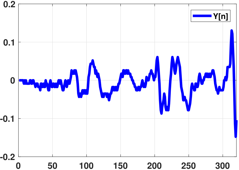
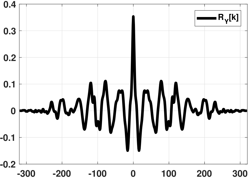
R_Y[k] = \E[Y[n+k]Y[n]] \approx \frac{1}{N}\sum_{n=1}^N Y[n+k]Y[n].

The averaging on the right-hand side is often done using xcorr in MATLAB or np.correlate in Python. A graphical illustration of the input and the autocorrelation function is shown in Figure 10.25.

**Figure 10.25.** An example time-series and its autocorrelation function.

After we have found $R_Y[k]$, we need to construct the Yule-Walker equation. For this linear prediction problem, the left-hand side of the Yule-Walker equation is the vector $\vr$, defined according to Eq. (10.44). The Yule-Walker equation also requires the matrix $\mR$. This $\mR$ can be constructed via the Toeplitz matrix as

\mR = \text{Toeplitz}\bigg\{R_Y[0],R_Y[1],\ldots,R_Y[K-1]\bigg\}.

In MATLAB, we can call Toeplitz to construct the matrix. In Python, the command is lin.Toeplitz.

To solve the Yule-Walker equation, we need to invert the matrix $\mR$. There are built-in commands for such an operation. In MATLAB, the command is \ (the backslash), whereas in Python the command is np.linalg.lstsq.

MATLAB

% MATLAB code to solve the Yule Walker Equation
    y = load('data_ch10.txt');
    K = 10;
    N = 320;
    
    y_corr = xcorr(y);
    R      = Toeplitz(y_corr(N+[0:K-1]));
    lhs    = y_corr(N+[1:K]);
    h      = R\lhs;

Python

# Python code to solve the Yule Walker Equation
    y = np.loadtxt('./data_ch10.txt')
    K = 10
    N = 320
    
    y_corr = np.correlate(y,y,mode='full')
    R      = lin.Toeplitz(y_corr[N-1:N+K-1]) #call scipy.linalg
    lhs    = y_corr[N:N+K]
    h      = np.linalg.lstsq(R,lhs,rcond = None)[0]

Note that in both the MATLAB and Python codes the Toeplitz matrix $\mR$ starts with the index $N$. This is because, as you can see from Figure 10.25, the origin of the autocorrelation function is the middle index of the computed autocorrelation function. For $\vr$, the starting index is $N+1$ because the vector starts with $R_Y[1]$.

To predict the future samples, we recall the autoregressive model for this problem:

\widehat{Y}[n] = \sum_{k=1}^{K} h[k]Y[n-k].

Therefore, given $Y[n-1],Y[n-2],\ldots,Y[n-K]$, we can predict $\widehat{Y}[n]$. Then we insert this predicted $\widehat{Y}[n]$ into the sequence and increment the estimation problem to the next time index. By repeating the process, we will be able to predict the future samples of $Y[n]$.

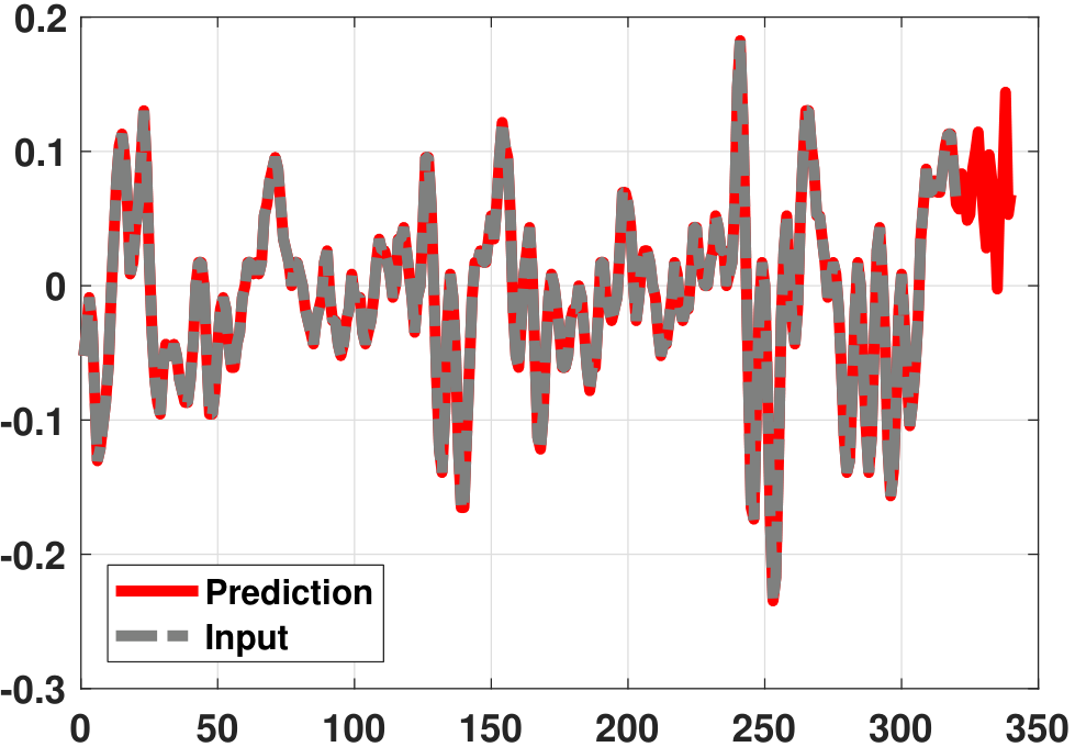
Figure 10.26 illustrates the prediction results of the Yule-Walker equation. As you can see, the predictions are reasonably meaningful since the patterns follow the trend.

The MATLAB and Python codes are shown below.

MATLAB

% MATLAB code to predict the samples
    z    = y(311:320);
    yhat = zeros(340,1);
    yhat(1:320) = y;
    
    for t = 1:20
        predict     = z'*h;
        z           = [z(2:10); predict];
        yhat(320+t) = predict;
    end
    
    plot(yhat, 'r', 'LineWidth', 3); hold on;
    plot(y,    'k', 'LineWidth', 4);

Python

# Python code to predict the samples
    z = y[310:320]
    yhat = np.zeros((340,1))
    yhat[0:320,0] = y
    
    for t in range(20):
      predict = np.inner(np.reshape(z,(1,10)),h)
      z = np.concatenate((z[1:10], predict))
      yhat[320+t,0] = predict
    
    plt.plot(yhat,'r')
    plt.plot(y,'k')
    plt.show()

10.6.5Wiener filter

In the previous formulation, we notice that the impulse response has a finite length. There are, however, problems in which the impulse response is infinite. For example, a recursive filter $h[n]$ will be infinitely long. The extension from finite length to infinite length is straightforward. We can model the problem as

\begin{aligned} Y[n] = \sum_{k=-\infty}^\infty h[k]X[n-k] + E[n]. \end{aligned}

However, when $h[n]$ is infinitely long the Yule-Walker equation does not hold because the matrix $\mR$ will be infinitely large. Nevertheless, the building block equation for Yule-Walker is still valid:

R_{YX}[i] = \sum_{k=-\infty}^{\infty} h[k] R_X[i-k].

To maintain the spirit of the Yule-Walker equation while enabling computation, we recognize that the infinite sum on the right-hand side is, in fact, a convolution. Thus we can take the (discrete-time) Fourier transform of both sides to obtain

S_{YX}(e^{j\omega}) = H(e^{j\omega}) S_X(e^{j\omega}).

Therefore, the corresponding optimal linear filter (in the Fourier domain) is

H(e^{j\omega}) = \frac{S_{YX}(e^{j\omega})}{S_X(e^{j\omega})},

and

h[n] = \mathcal{F}^{-1} \left\{\frac{S_{YX}(e^{j\omega})}{S_X(e^{j\omega})}\right\}.

The filter obtained in this way is known as the Wiener filter.

Example 10.21

(Denoising) Suppose $X[n] = Y[n] + W[n]$, where $W[n]$ is the noise term that is independent of $Y[n]$, as shown in Figure 10.27.

Now, given the input function $X[n]$, can we construct the Wiener filter $h[n]$ such that the predicted function $\widehat{Y}[n]$ is as close to $Y[n]$ as possible? The Wiener filter for this problem is also the optimal denoising filter.

Solution

The following correlation functions can easily be seen:

\begin{aligned} R_{X}[k] &= \E[X[n+k]X[n]] \\ &= \E[(Y[n+k]+W[n+k])(Y[n]+W[n])]\\ &= \E[Y[n+k]Y[n]] + \E[Y[n+k]W[n]] \\ &\qquad + \E[W[n+k]Y[n]] + \E[W[n+k]W[n]]\\ &= \E[Y[n+k]Y[n]] + 0 + 0 + \E[W[n+k]W[n]]\\ &= R_Y[k] + R_{W}[k]. \end{aligned}

Similarly, we have

\begin{aligned} R_{YX}[k] &= \E[Y[n+k]X[n]] \\ &= \E[Y[n+k](Y[n]+W[n])] = R_Y[k]. \end{aligned}

Consequently, the optimal linear filter is

\begin{aligned} H(e^{j\omega}) &= \frac{S_{YX}(e^{j\omega})}{S_X(e^{j\omega})} \\ &= \frac{\calF\{R_{YX}[k]\}}{\calF\{R_{X}[k]\}}\\ &= \frac{S_{Y}(e^{j\omega})}{S_Y(e^{j\omega}) + S_{W}(e^{j\omega})}. \end{aligned}

What is the Wiener filter for a denoising problem?

Suppose the corrupted function $X[n]$ is related to the clean function $Y[n]$ through $X[n] = Y[n] + W[n]$, for some noise function $W[n]$.
The Wiener filter is
$H(e^{j\omega}) = \frac{S_{Y}(e^{j\omega})}{S_Y(e^{j\omega}) + S_{W}(e^{j\omega})}.$
To perform the filtering, the denoised function $\widehat{Y}[n]$ is
$\widehat{Y}[n] = \calF^{-1}\left\{ H(e^{j\omega}) X(e^{j\omega})\right\}.$

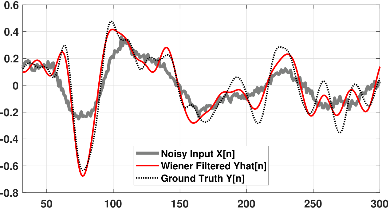
Figure 10.28 shows an example of applying the Wiener filter to a noise removal problem. In this example we let $W[n]$ be an i.i.d. Gaussian process with standard deviation $\sigma = 0.05$ and mean $\mu = 0$. The noisy samples of random process $X[n]$ are defined as $X[n] = Y[n] + W[n]$, where $Y[n]$ is the clean function. As you can see from Figure 10.28(a), the Wiener filter is able to denoise the function reasonably well.

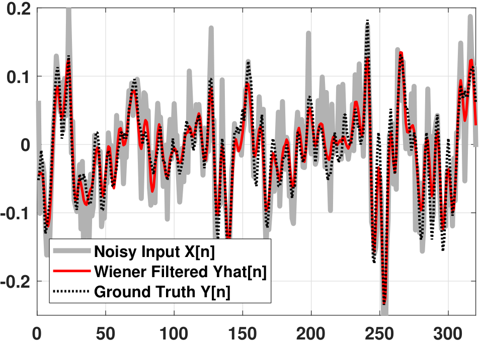
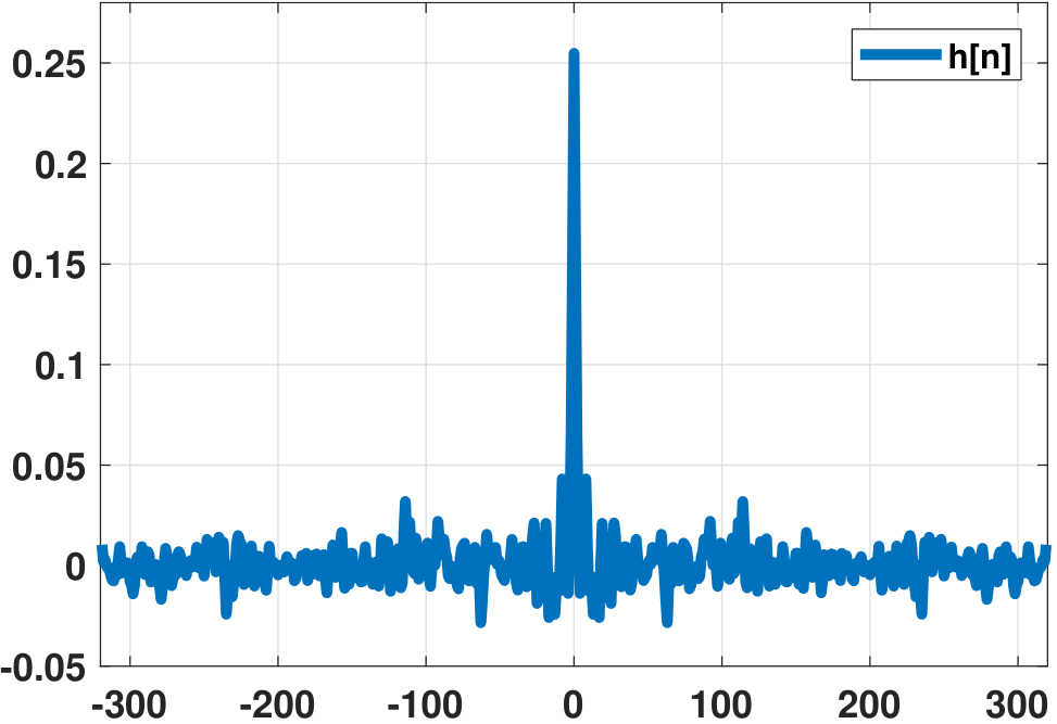
**Figure 10.28.** (a) Applying a Wiener filter to denoise a function. (b) The Wiener filter used for the denoising task.

The optimal linear filter used for this denoising task is infinitely long. This can be seen in Figure 10.28(b), where the filter length is the same as the length of the observed time series $X[n]$. If $X[n]$ is longer, the filter $h[n]$ will also become longer. Therefore, finite-length approaches such as the Yule-Walker equation do not apply here.

The MATLAB / Python codes used to generate Figure 10.28(a) are shown below. The main commands here are scipy.fft and scipy.ifft, which are available in the scipy library. The commands Yhat = H.*fft(x, 639) in MATLAB execute the Wiener filtering step. Here, we resample the function x to 639 samples so that it matches with the Wiener filter H. Similar commands in Python are H * fft(x, 639).

MATLAB

% MATLAB code for Wiener filtering
    w = 0.05*randn(320,1);
    x = y + w;
    
    Ry = xcorr(y);
    Rw = xcorr(w);
    Sy = fft(Ry);
    Sw = fft(Rw);
    H = Sy./(Sy + Sw);
    Yhat = H.*fft(x, 639);
    yhat = real(ifft(Yhat));
    
    plot(x, 'LineWidth', 4, 'Color', [0.7, 0.7, 0.7]); hold on;
    plot(yhat(1:320), 'r', 'LineWidth', 2);
    plot(y, 'k:', 'LineWidth', 2);

Python

# Python code for Wiener filtering
    from scipy.fft import fft, ifft
    w = 0.05*np.random.randn(320)
    x = y + w
    
    Ry = np.correlate(y,y,mode='full')
    Rw = np.correlate(w,w,mode='full')
    Sy = fft(Ry)
    Sw = fft(Rw)
    H  = Sy / (Sy+Sw)
    Yhat = H * fft(x, 639)
    yhat = np.real(ifft(Yhat))
    
    plt.plot(x,color='gray')
    plt.plot(yhat[0:320],'r')
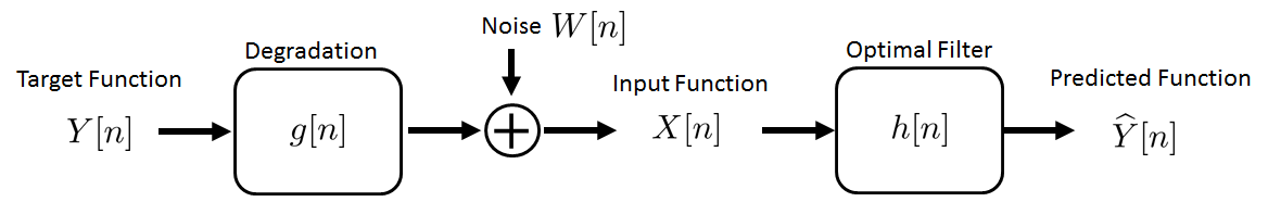
    plt.plot(y,'k:')

Example 10.22

(Deconvolution) Suppose that the corrupted function is generated according to a linear process given by

\begin{aligned} X[n] = \sum_{\ell=-\infty}^{\infty} g[\ell] Y[n-\ell] + W[n], \end{aligned}

where $g[n]$ is the impulse response of some kind of degradation process and $W[n]$ is the Gaussian noise term, as shown in Figure 10.29. Find the optimal linear filter (i.e., the Wiener filter) to estimate $\widehat{Y}[n]$.

Solution

To construct the Wiener filter, we first determine the cross-correlation function:

\begin{aligned} R_{YX}[k] &= \E\left[Y[n+k]X[n]\right] = \E\left[Y[n+k] \left(\sum_{\ell=-\infty}^{\infty} g[\ell]Y[n-\ell] + W[n]\right)\right]. \end{aligned}

Using algebra, it follows that

\begin{aligned} &\E\left[Y[n+k] \left(\sum_{\ell=-\infty}^{\infty} g[\ell]Y[n-\ell] + W[n]\right)\right]\\ &= \sum_{\ell=-\infty}^{\infty} g[\ell] \E[Y[n+k] Y[n-\ell]] + \E[Y[n+k]W[n]]\\ &= \sum_{\ell=-\infty}^{\infty} g[\ell] R_Y[k+\ell] + 0 = (g \circledast R_Y)[k], \end{aligned}

which is the correlation between $g$ and $R_Y$. Therefore, the cross power spectral density $S_{YX}(e^{j\omega})$ is

\begin{aligned} S_{YX}(e^{j\omega}) = \overline{G(e^{j\omega})}S_Y(e^{j\omega}). \end{aligned}

The autocorrelation of this problem is

\begin{aligned} R_{X}[k] &= \E\left[X[n+k]X[n]\right] \\ &= \E\left[ ((g\ast Y)[n+k] + W[n+k]) ((g\ast Y)[n] + W[n])\right]\\ &= \E\left[ (g\ast Y)[n+k] (g\ast Y)[n] \right] + \E[W[n+k]W[n]]\\ &= (g \circledast (g \ast R_Y))[k] + R_W[k], \end{aligned}

where, according to the previous section, the first part is the correlation $\circledast$ followed by a convolution $\ast$. Therefore, the power spectral density of $X$ is

\begin{aligned} S_{X}(e^{j\omega}) = |G(e^{j\omega})|^2 S_Y(e^{j\omega}) + S_W(e^{j\omega}). \end{aligned}

Combining the results, the Wiener filter is

\begin{aligned} H(e^{j\omega}) &= \frac{S_{YX}(e^{j\omega})}{S_X(e^{j\omega})} = \frac{\overline{G(e^{j\omega})}S_Y(e^{j\omega})}{|G(e^{j\omega})|^2 S_Y(e^{j\omega}) + S_W(e^{j\omega})}. \end{aligned}

What is the Wiener filter for a deconvolution problem?

Suppose that the corrupted function $X[n]$ is related to the clean function $Y[n]$ through $X[n] = (g \ast Y)[n] + W[n]$, for some degradation $g[n]$ and noise $W[n]$.
The Wiener filter is
$H(e^{j\omega}) = \frac{\overline{G(e^{j\omega})}S_Y(e^{j\omega})}{|G(e^{j\omega})|^2 S_Y(e^{j\omega}) + S_W(e^{j\omega})}.$
To perform the filtering, the estimated function $\widehat{Y}[n]$ is
$\widehat{Y}[n] = \calF^{-1}\left\{ H(e^{j\omega}) X(e^{j\omega})\right\}.$

As an example of the deconvolution problem, we show a WSS function $Y[n]$ in Figure 10.30. This clean function $Y[n]$ is constructed by passing an i.i.d. noise process through an arbitrary LTI system so that the WSS property is guaranteed. Given this $Y[n]$, we construct a degradation process in which the impulse response is given by $g[n]$. In this example, we assume that $g[n]$ is a uniform function. We then add noise $W[n]$ to the time series to obtain the corrupted observation $X[n]$. The reconstruction by the Wiener filter is shown in Figure 10.30.

The MATLAB and Python codes used to generate Figure 10.30 are shown below.

MATLAB

% MATLAB code to solve the Wiener deconvolution problem
    load('ch10_wiener_deblur_data');
    g = ones(32,1)/32;
    w = 0.02*randn(320,1);
    x = conv(y,g,'same') + w;
    
    Ry = xcorr(y);
    Rw = xcorr(w);
    Sy = fft(Ry);
    Sw = fft(Rw);
    G  = fft(g,639);
    
    H = (conj(G).*Sy)./(abs(G).^2.*Sy + Sw);
    Yhat = H.*fft(x, 639);
    yhat = real(ifft(Yhat));
    
    figure;
    plot(x, 'LineWidth', 4, 'Color', [0.5, 0.5, 0.5]); hold on;
    plot(16:320+15, yhat(1:320), 'r', 'LineWidth', 2);
    plot(1:320, y, 'k:', 'LineWidth', 2);

Python

# Python code to solve the Wiener deconvolution problem
    y = np.loadtxt('./ch10_wiener_deblur_data.txt')
    g = np.ones(64)/64
    w = 0.02*np.random.randn(320)
    x = np.convolve(y,g,mode='same') + w
    
    Ry = np.correlate(y,y,mode='full')
    Rw = np.correlate(w,w,mode='full')
    Sy = fft(Ry)
    Sw = fft(Rw)
    G  = fft(g,639)
    H = (np.conj(G)*Sy)/( np.power(np.abs(G),2)*Sy + Sw )
    
    Yhat = H * fft(x, 639)
    yhat = np.real(ifft(Yhat))
    
    plt.plot(x,color='gray')
    plt.plot(np.arange(32,320+32),yhat[0:320],'r')
    plt.plot(y,'k:')

Caveat to Wiener filtering. In practice, the above Wiener filter needs to be modified because $S_Y(e^{j\omega})$ and $S_W(e^{j\omega})$ cannot be estimated from the data via the temporal correlation (as we did in the MATLAB/Python programs). The reason is that we never have access to $Y[n]$ and $W[n]$. In this case, one has to guess the power spectral densities $S_Y(e^{j\omega})$ and $S_W(e^{j\omega})$. The noise power $S_W(e^{j\omega})$ is usually not difficult to estimate. For example, in the program we showed above, the noise power spectral density is Sw = 0.02^2*320 (MATLAB), which is the noise variance times the number of samples.

The signal $S_Y(e^{j\omega})$ is often the hard part. In the absence of any knowledge about the ground truth's power spectral density, the Wiener filter does not work. However, for certain problems in which $S_Y(e^{j\omega})$ can be predetermined by prior knowledge, the Wiener filter is guaranteed to be optimal — optimal in the mean-squared-error sense over the entire time axis.

Wiener filter versus ridge regression. The Wiener filter equation can be interpreted as a ridge regression. Denoting the forward observation model by

\vx = \mG \vy + \vw,

the corresponding ridge regression minimization is

\begin{aligned} \vyhat &= \argmin{\vy} \;\; \|\vx - \mG\vy\|^2 + \lambda \|\vy\|^2 \\ &= (\mG^T\mG + \lambda\mI)^{-1}\mG^T\vx. \end{aligned}

If $\mG$ is a convolutional matrix, the above solution can be written in the Fourier domain (by using the Fourier transform as the eigenvectors):

\widehat{Y}(e^{j\omega}) = \underset{H(e^{j\omega})}{\underbrace{\left[\frac{\overline{G(e^{j\omega})}}{|G(e^{j\omega})|^2 + \lambda}\right]}} X(e^{j\omega}).

Comparing this “optimal linear filter” with the Wiener filter, we observe that the Wiener filter has slightly more generality:

\widehat{Y}(e^{j\omega}) = \left[\frac{\overline{G(e^{j\omega})} \textcolor{blue}{S_Y(e^{j\omega})}}{|G(e^{j\omega})|^2 \textcolor{blue}{S_Y(e^{j\omega})} + \textcolor{blue}{S_W(e^{j\omega})}} \right] X(e^{j\omega}).

Therefore, in the absence of $S_Y(e^{j\omega})$ and assuming that $S_W(e^{j\omega})$ is a constant (e.g., for Gaussian noise), the Wiener filter is exactly a ridge regression.