eBook › Chapter 10 · Random Processes

Section 10.4

Power Spectral Density

Beginning with this section we are going to focus on WSS processes. By WSS, we mean that the autocorrelation function \(R_X(t_1,t_2)\) has a Toeplitz structure. Putting it in other words, we assume \(R_X(t_1,t_2)\) can be simplified to \(R_X(\tau)\), where \(\tau = t_1 - t_2\). We call this property time invariance.

10.4.1Basic concepts

Assuming that \(R_X(\tau)\) is square integrable, i.e., \(\int_{-\infty}^{\infty} R_X(\tau)^2\; d\tau < \infty\), we can now define the Fourier transform of \(R_X(\tau)\) which is called the power spectral density.

Theorem 10.2 (Einstein-Wiener-Khinchin Theorem)

The power spectral density \(S_X(\omega)\) of a WSS process is

\begin{aligned} S_X(\omega) &= \int_{-\infty}^\infty R_X(\tau)\; e^{-j \omega \tau}\; d\tau \\ &= \mathcal{F}(R_X(\tau)), \end{aligned}

assuming that \(\int_{-\infty}^{\infty} R_X(\tau)^2\; d\tau < \infty\) so that the Fourier transform of \(R_X(\tau)\) exists.

Practice Exercise 10.4

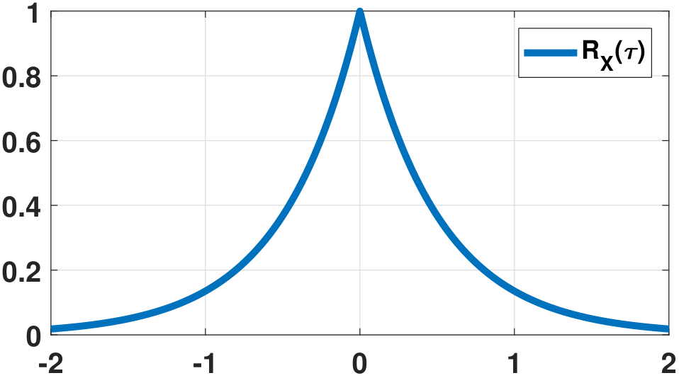
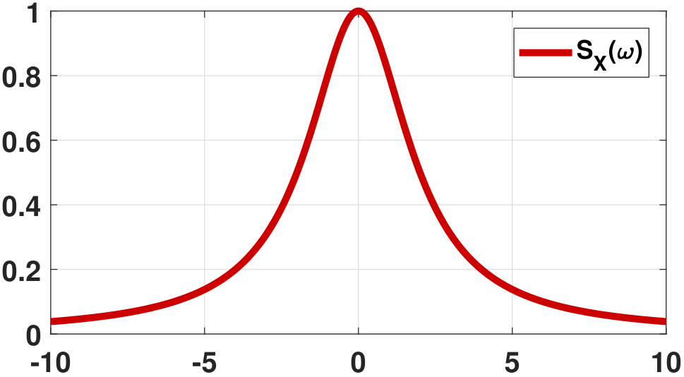
Let \(R_X(\tau)=e^{-2\alpha |\tau|}\). Find \(S_X(\omega)\).

Solution

Using the Fourier transform table,

S_X(\omega)=\mathcal{F}\left\{R_X(\tau)\right\}=\frac{4\alpha}{4\alpha^2+\omega^2}.

Figure 10.17 shows \(R_X(\tau)\) and \(S_X(\omega)\).

**Figure 10.17.** Example for \(R_X(\tau)=e^{-2\alpha |\tau|}\), with \(\alpha = 1\).

Why is Theorem thm: ch10 Wie a theorem rather than a definition? This is because power spectral density has its definition. There is no way that you can get any “power” information merely by looking at the Fourier transform of \(R_X(\tau)\). We will discuss the origin of the power spectral density later, but for now, we only need to know that \(S_X(\omega)\) is the Fourier transform of \(R_X(\tau)\).

Remark. The power spectral density is defined for WSS processes. If the process is not WSS, then \(R_X\) will be a 2D function instead of a 1D function of \(\tau\), so we cannot take the Fourier transform in \(\tau\). We will discuss this in detail shortly.

Practice Exercise 10.5

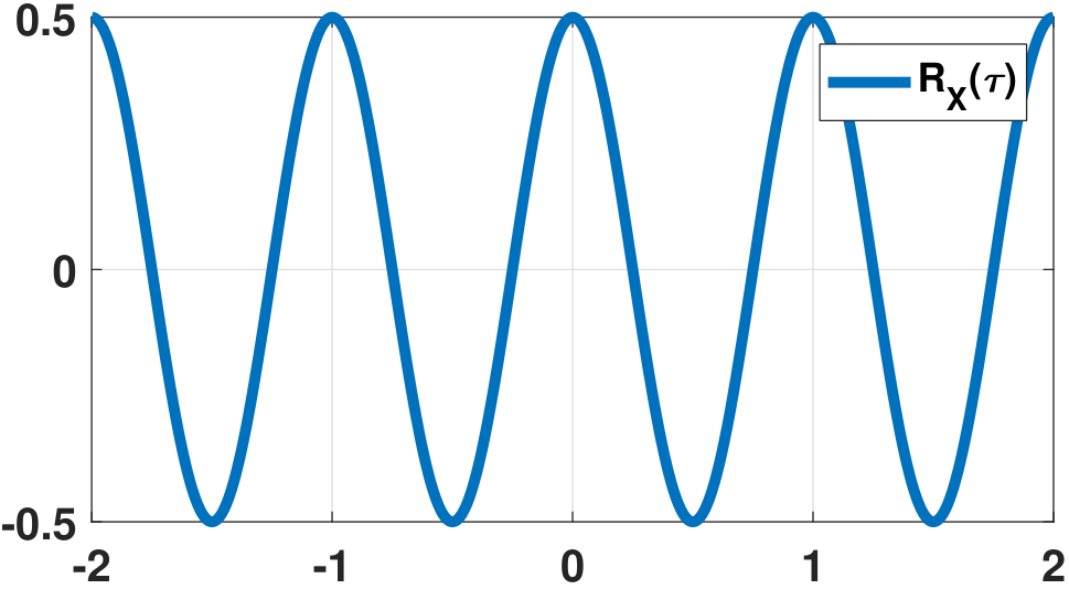
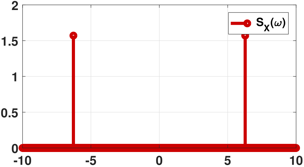
Let \(X(t)=a\cos(\omega_0 t+\Theta), \; \Theta\sim\) Uniform\([0,2\pi]\). Find \(S_X(\omega)\).

Solution

We know that the autocorrelation function is

\begin{aligned} R_X(\tau) &=\frac{a^2}{2}\cos(\omega_0 \tau) =\frac{a^2}{2} \left(\frac{e^{j \omega_0 \tau}+e^{-j \omega_0 \tau}}{2}\right). \end{aligned}

By taking the Fourier transform of both sides, we have

\begin{aligned} S_X(\omega) &=\frac{a^2}{2} \left[\frac{2\pi \delta(\omega-\omega_0)+2\pi\delta(\omega+\omega_0)}{2}\right] \\ &=\frac{\pi a^2}{2} \left[\delta(\omega-\omega_0)+\delta(\omega+\omega_0)\right]. \end{aligned}

The result is shown in Figure 10.18.

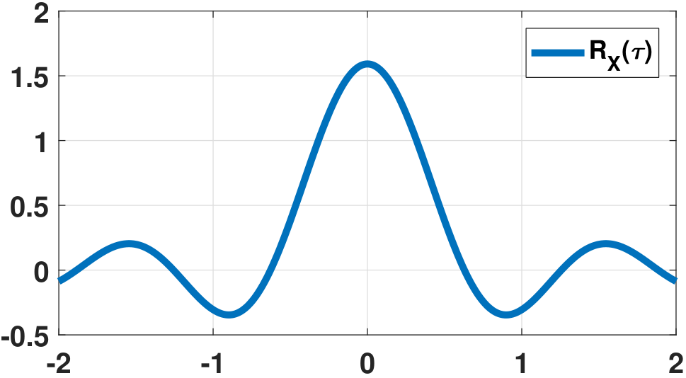
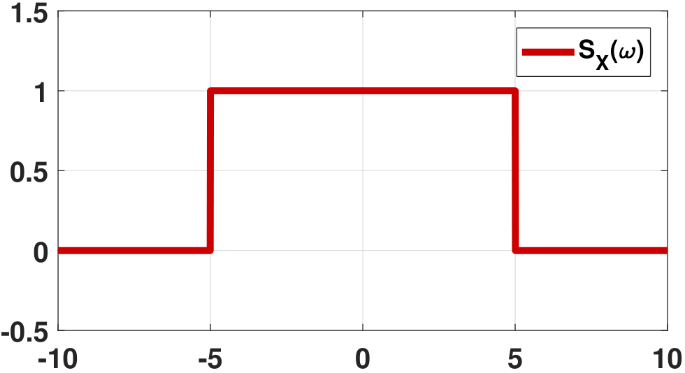
**Figure 10.18.** Example for \(R_X(\tau)=\frac{a^2}{2}\cos(\omega_0 \tau)\), with \(a = 1\) and \(\omega_0 = 2\pi\).

Practice Exercise 10.6

Let \(S_X(\omega)=\frac{N_0}{2} \textrm{rect}(\frac{\omega}{2W})\). Find \(R_X(\tau)\).

Solution

Since \(S_X(\omega) = \calF(R_X(\tau))\), the inverse holds:

R_X(\tau)= \frac{N_0}{2} \frac{W}{\pi} \textrm{sinc}(W\tau).

This example shows what we call the bandlimited white noise. The power spectral density \(S_X(\omega)\) is uniform, meaning that it covers all frequencies (or wavelengths in optics). It is called “white noise” because white light is essentially a mixture of all wavelengths.

The bandwidth of the power spectral density \(W\) defines the zero crossings of \(R_X(\tau)\). It is easy to show that when \(W \rightarrow \infty\), \(R_X(\tau)\) converges to a delta function. This happens when \(X(t)\) is i.i.d. Gaussian. Therefore, the pure Gaussian noise random process is also known as the white noise process. Reshaping the i.i.d. Gaussian noise to an arbitrary power spectral density can be done by passing it through a linear filter, as we will explain later.

**Figure 10.19.** Example for \(S_X(\omega)=\frac{N_0}{2} \textrm{rect}(\frac{\omega}{2W})\), with \(N_0 = 2\) and \(W = 5\).

Finding \(S_X(\omega)\) from \(R_X(\tau)\) is straightforward, at least in principle. The more interesting questions to ask are: (1) Why do we need to learn about power spectral density? (2) Why do we need WSS to define power spectral density?

How is power spectral density useful?

sep0ex
Power spectral densities are useful when we pass a random process through some linear operations, e.g., convolution, running average, or running difference.
Power spectral densities are the Fourier transforms of the autocorrelation functions. Fourier transforms are useful for speeding up computation and drawing random samples from a given power spectral density.

A random process itself is not interesting until we process it; there are many ways to do this. The most basic operation is to send the random process through a linear time-invariant system, e.g., a convolution. Convolution is equivalent to filtering the random process. For example, if the input process contains noise, we can design a linear time-invariant filter to denoise the random process. The power spectral density, which is the Fourier transform of the autocorrelation function, makes the filtering easier because everything can be done in the spectral (Fourier) domain. Moreover, we can analyze the performance and quantify the limit using standard results in Fourier analysis. For some specialized problems such as imaging through atmospheric turbulence, the distortions happen in the phase domain. This can be simulated by drawing samples from the power spectral density, e.g., the Kolmogorov spectrum or the von K\'arm\'an spectrum. Power spectral densities have many important engineering applications.

Why does the power spectral density require wide-sense stationarity?

sep0ex
If a process is WSS, then \(R_X\) will have a Toeplitz structure.
A Toeplitz matrix is important. If you do eigendecomposition of a Toeplitz matrix, the eigenvectors are the Fourier bases.
So if \(R_X\) is Toeplitz, then you can diagonalize it using the Fourier transform.
Therefore, the power spectral density can be defined.

Why does power spectral density require WSS? This has to do with the Toeplitz structure of the autocorrelation function. To make our discussion easier let us discretize the autocorrelation function \(R_X(t_1,t_2)\) by considering \(R_X[m,n]\). (You can do a mental calculation by converting \(t_1\) to integer indices \(m\), and \(t_2\) to \(n\). See any textbook on signals and systems if you need help. This is called the “discrete-time signal”.) Following the range of \(t_1\) and \(t_2\), \(R_X[m,n]\) can be expressed as:

\begin{aligned} \mR = \begin{bmatrix} R_X[0] & R_X[1] & \cdots & R_X[N-1]\\ R_X[1] & R_X[0] & \cdots & R_X[N-2]\\ \vdots & \vdots & \ddots & \vdots \\ R_X[N-1] & R_X[N-2] & \cdots & R_X[0]\\ \end{bmatrix}, \end{aligned}

where we used the fact that \(R_X[m,n] = R_X[m-n]\) for WSS processes and \(R_X[k] = R_X[-k]\). We call the resulting matrix \(\mR\) the autocorrelation matrix, which is a discretized version of the autocorrelation function \(R_X(t_1,t_2)\). Looking at \(\mR\), we again observe the Toeplitz structure. For example, Figure 10.20 shows one Toeplitz structure and one non-Toeplitz structure.

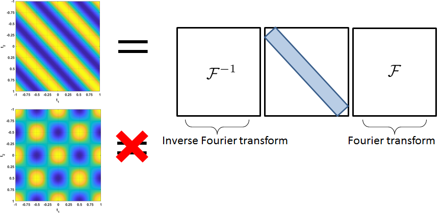
**Figure 10.20.** We show two autocorrelation functions \(R_{X}[m,n]\) on the left-hand side. The first autocorrelation function comes from a WSS process that has a Toeplitz structure. The second autocorrelation function does not have Toeplitz structure. For the Toeplitz matrix, we can diagonalize it using the Fourier transform. The eigenvalues are the power spectral density.

Any Toeplitz matrix \(\mR\) can be diagonalized using the Fourier transforms. That is, we can write \(\mR\) as

\mR = \mF^H\mLambda\mF,

where \(\mF\) is the (discrete) Fourier transform matrix and \(\mLambda\) is a diagonal matrix. This can be understood as the eigendecomposition of \(\mR\). The important point here is that only Toeplitz matrices can be eigendecomposed using the Fourier transform; an arbitrary symmetric matrix cannot. Figure 10.20 illustrates this point. If your matrix is Toeplitz, you can diagonalize it, and hence you can define the power spectral density, just as in the first example. If your matrix is not Toeplitz, then the power spectral density is undefined. To get the Toeplitz matrix, you must start with a WSS process.

Before moving on, we define cross power spectral densities, which will be useful in some applications.

Definition 10.9

The cross power spectral density between two random processes \(X(t)\) and \(Y(t)\) is

\begin{array}{lll} S_{X,Y}(\omega)=\mathcal{F}(R_{X,Y}(\tau)) & \textrm{where} & R_{X,Y}(\tau)=\E[X(t+\tau)Y(t)], \\ S_{Y,X}(\omega)=\mathcal{F}(R_{Y,X}(\tau)) & \textrm{where} & R_{Y,X}(\tau)=\E[Y(t+\tau)X(t)]. \end{array}

Remark. In general, \(S_{X,Y}(\omega) \neq S_{Y,X}(\omega)\). Rather, since \(R_{X,Y}(\tau)=R_{Y,X}(-\tau)\), we have \(S_{X,Y}(\omega) = \overline{S_{Y,X}(\omega)}\).

10.4.2Origin of the power spectral density

To understand the power spectral density, it is crucial to understand where it comes from and why it is the Fourier transform of the autocorrelation function.

We begin by assuming that \(X(t)\) is a WSS random process with mean \(\mu_X\) and autocorrelation \(R_X(\tau)\). We now consider the notion of power. Consider a random process \(X(t)\). The power within a period \([-T,T]\) is

\widehat{P}_X = \frac{1}{2T} \int_{-T}^T |X(t)|^2 \;dt.

\(\widehat{P}_X\) defines the power because the integration alone is the energy, and the normalization by \(1/2T\) gives us the power. However, there are two problems. First, since \(X(t)\) is random, the power \(\widehat{P}_X\) is also random. Is there a way we can eliminate the randomness? Second, \(T\) is a finite period of time. It does not capture the entire process, and so we do not know the power of the entire process.

A natural solution to these two problems is to consider

P_X \bydef \E\left[\lim_{T \rightarrow \infty} \frac{1}{2T} \int_{-T}^T |X(t)|^2 \;dt\right].

Here, we take the limit of \(T\) to infinity so that we can compute the power of the entire process. We also take the expectation to eliminate the randomness. Therefore, \(P_X\) can be regarded as the average power of the complete random process \(X(t)\).

Next, we need one definition and one lemma. The definition defines \(S_X(\omega)\), and the lemma will link \(S_X(\omega)\) with the power \(P_X\).

Definition 10.10

The power spectral density (PSD) of a WSS process is defined as

S_X(\omega)=\lim_{T \rightarrow \infty} \frac{\E\left[|\widetilde{X}_T(\omega)|^2\right]}{2T},

where

\widetilde{X}_T(\omega)=\int_{-T}^T X(t)e^{-j \omega t} \;dt

is the Fourier transform of \(X(t)\) limited to \([-T,T]\).

This definition is abstract, but in a nutshell, it simply considers everything in the Fourier domain. The ratio \(|\widetilde{X}_T(\omega)|^2/2T\) is the power, but in the frequency domain. The reason is that if \(X(t)\) is Fourier transformable, then Parseval's theorem will hold. Parseval's theorem states that energy in the original space is conserved in the Fourier space. Since the ratio \(|\widetilde{X}_T(\omega)|^2/2T\) is the energy divided by time, it is the power. However, this is still not enough to help us understand power spectral density: We need a lemma.

Lemma 10.2

Define

P_X \bydef \E\left[\lim_{T \rightarrow \infty} \frac{1}{2T} \int_{-T}^T |X(t)|^2 \;dt\right].

Then

P_X = \frac{1}{2\pi} \int_{-\infty}^\infty S_X(\omega) \;d\omega.

The lemma has to be read together with the previous definition. If we can prove the lemma, we know that by integrating \(S_X(\omega)\) we will obtain the power. Therefore, \(S_X(\omega)\) can be viewed as a density function, specifically the density function of the power. \(S_X(\omega)\) is called the power spectral density because everything is defined in the Fourier domain. Putting this all together gives us “power spectral density”.

Proof. First, we recall that \(P_X\) is the expectation of the average power of \(X(t)\). Let

X_T(t)=\left\{ \begin{array}{ll} X(t) & -T \leq t \leq T, \\ 0 & \textrm{otherwise}. \end{array} \right.

It follows that integrating over \(-\infty\) to \(\infty\) is equivalent to

\int_{-\infty}^\infty |X_T(t)|^2 \;dt = \int_{-T}^T |X(t)|^2 \;dt.

By Parseval's theorem, energy is conserved in both the time and the frequency domain:

\int_{-\infty}^\infty |X_T(t)|^2 \;dt = \frac{1}{2\pi} \int_{-\infty}^\infty |\widetilde{X}_T(\omega)|^2 \;d\omega.

Therefore, \(P_X\) satisfies

\begin{aligned} P_X = \E\left[\lim_{T \rightarrow \infty} \frac{1}{2T} \int_{-T}^T |X(t)|^2 \;dt\right] &= \E\left[\lim_{T \rightarrow \infty} \frac{1}{2\pi} \frac{1}{2T} \int_{-\infty}^\infty |\widetilde{X}_T(\omega)|^2 \;d\omega\right] \\ &=\frac{1}{2\pi} \int_{-\infty}^\infty \underbrace{\lim_{T \rightarrow \infty} \frac{1}{2T} \E\left[|\widetilde{X}_T(\omega)|^2\right]}_{\bydef S_X(\omega)} \; d\omega. \end{aligned}

■

The power spectral densities are functions whose integrations give us the power. If we want to determine the power of a random process, the Einstein-Wiener-Khinchin theorem (Theorem thm: ch10 Wie) says that \(S_X(\omega)\) is just the Fourier transform of \(R_X(\tau)\):

\begin{aligned} S_X(\omega) = \int_{-\infty}^\infty R_X(\tau)\; e^{-j \omega \tau}\; d\tau = \mathcal{F}(R_X(\tau)). \end{aligned}

The proof of the Einstein-Wiener-Khinchin theorem is quite intricate, so we defer the proof to the Appendix. The significance of the theorem is that it turns an abstract quantity, the power spectral density, into a very easily computable quantity, namely the Fourier transform of the autocorrelation function. For now, we will happily use this theorem because it saves us a great deal of trouble when we want to determine the power spectral density from first principles.