eBook › Chapter 4 · Continuous Random Variables

Section 4.3

Cumulative Distribution Function

When we discussed discrete random variables, we introduced the concept of cumulative distribution functions (CDFs). One of the motivations was that if we view a PMF as a train of delta functions, they are technically not well-defined functions. However, it turns out that the CDF is always a well-defined function. In this section, we will complete the story by first discussing the CDF for continuous random variables. Then, we will come back and show you how the CDF can be derived for discrete random variables.

4.3.1CDF for continuous random variables

Definition 4.7

Let $X$ be a continuous random variable with a sample space $\Omega = \R$. The cumulative distribution function (CDF) of $X$ is

F_X(x) \bydef \Pb[X \le x] = \int_{-\infty}^{x} f_X(x') \;dx'.

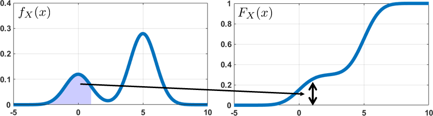
The interpretation of the CDF can be seen from Figure 4.5. Given a PDF $f_X$, the CDF $F_X$ evaluated at $x$ is the integration of $f_X$ from $-\infty$ up to a point $x$. The integration of $f_X$ from $-\infty$ to $x$ is nothing but the area under the curve of $f_X$. Since $f_X$ is non-negative, the larger the value $x$ at which we evaluate $F_X(x)$, the more area under the curve we are looking at. In the extreme when $x = -\infty$, we can see that $F_X(-\infty) = 0$, and when $x = +\infty$ we have that $F_X(+\infty) = \int_{-\infty}^{\infty} f_X(x) \;dx = 1$.

Practice Exercise 4.10

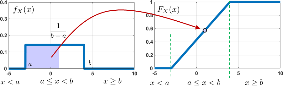
(Uniform random variable) Let $X$ be a continuous random variable with PDF $f_X(x) = \frac{1}{b-a}$ for $a \le x \le b$, and is 0 otherwise. Find the CDF of $X$.

Solution

The CDF of $X$ is given by

\begin{aligned} F_X(x) = \begin{cases} 0, &\quad x \le a,\\ \int_{-\infty}^{x} f_X(x') \;dx' = \int_{a}^x \frac{1}{b-a} \;dx' = \frac{x-a}{b-a}, &\quad a < x \le b,\\ 1, &\quad x > b. \end{cases} \end{aligned}

As you can see from this practice exercise, we explicitly break the CDF into three segments. The first segment gives $F_X(x) = 0$ because for any $x \le a$, there is nothing to integrate, since $f_X(x)=0$ for any $x \le a$. Similarly, for the last segment, $F_X(x) = 1$ for all $x > b$ because once $x$ goes beyond $b$, the integration will cover all the non-zeros of $f_X$. Figure 4.6 illustrates the PDF and CDF for this example.

In MATLAB, we can generate the PDF and CDF using the commands pdf and cdf respectively. For the particular example shown in Figure 4.6, the following code can be used. A similar set of commands can be implemented in Python.

MATLAB

% MATLAB code to generate the PDF and CDF
    unif = makedist('Uniform','lower',-3,'upper',4);
    x  = linspace(-5, 10, 1500)';
    f  = pdf(unif, x);
    F  = cdf(unif, x);
    figure(1); plot(x, f, 'LineWidth', 6);
    figure(2); plot(x, F, 'LineWidth', 6);

Python

# Python code to generate the PDF and CDF
    import numpy as np
    import matplotlib.pyplot as plt
    import scipy.stats as stats
    x = np.linspace(-5,10,1500)
    f = stats.uniform.pdf(x,-3,4)
    F = stats.uniform.cdf(x,-3,4)
    plt.plot(x,f); plt.show()
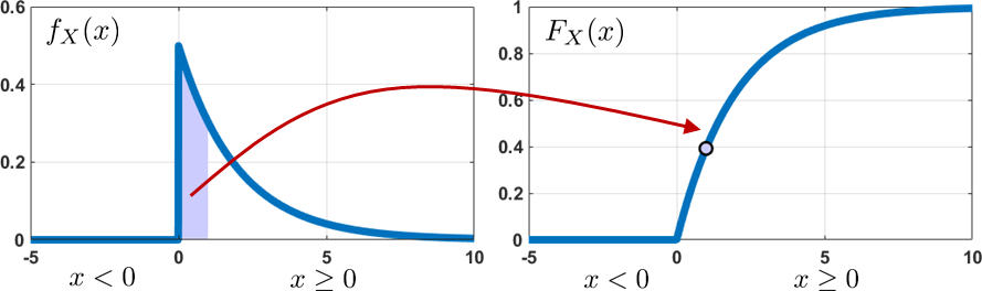
    plt.plot(x,F); plt.show()

Practice Exercise 4.11

(Exponential random variable) Let $X$ be a continuous random variable with PDF $f_X(x) = \lambda e^{-\lambda x}$ for $x \ge 0$, and 0 otherwise. Find the CDF of $X$.

Solution

Clearly, for $x < 0$, we have $F_X(x) = 0$. For $x \ge 0$, we can show that

\begin{aligned} F_X(x) = \int_{0}^{x} f_X(x')\;dx' = \int_{0}^{x} \lambda e^{-\lambda x'}\;dx' = 1-e^{-\lambda x}. \end{aligned}

Therefore, the complete CDF is (see Figure 4.7 for illustration):

F_X(x) = \begin{cases} 0, &\quad x < 0,\\ 1-e^{-\lambda x}, &\quad x \ge 0. \end{cases}

The MATLAB code and Python code to generate this figure are shown below.

MATLAB

% MATLAB code to generate the PDF and CDF
    pd = makedist('exp',2);
    x  = linspace(-5, 10, 1500)';
    f  = pdf(pd, x);
    F  = cdf(pd, x);
    figure(1); plot(x, f, 'LineWidth', 6);
    figure(2); plot(x, F, 'LineWidth', 6);

Python

# Python code to generate the PDF and CDF
    import numpy as np
    import matplotlib.pyplot as plt
    import scipy.stats as stats
    x = np.linspace(-5,10,1500)
    f = stats.expon.pdf(x,2)
    F = stats.expon.cdf(x,2)
    plt.plot(x,f); plt.show()
    plt.plot(x,F); plt.show()

4.3.2Properties of CDF

Let us now describe the properties of a CDF. If we compare these with those for the discrete cases, we see that the continuous cases simply replace the summations by integrations. Therefore, we should expect to inherit most of the properties from the discrete cases.

Proposition 4.1

Let $X$ be a random variable (either continuous or discrete), then the CDF of $X$ has the following properties:

(i) The CDF is nondecreasing.
(ii) The maximum of the CDF is when $x = \infty$: $F_X(+\infty) = 1$.
(iii) The minimum of the CDF is when $x = -\infty$: $F_X(-\infty) = 0$.

Proof. For (i), we notice that $F_X(x) = \int_{-\infty}^{x} f_X(x')\;dx'$. Therefore, if $s \le t$ then

\begin{aligned} F_X(s) = \int_{-\infty}^{s} f_X(x')\;dx' \le \int_{-\infty}^{t} f_X(x')\;dx' = F_X(t). \end{aligned}

Thus it shows that $F_X$ is nondecreasing. (It does not need to be increasing because a CDF can have a steady state.) For (ii) and (iii), we can show that

\begin{aligned} F_X(+\infty) &= \int_{-\infty}^{+\infty} f_X(x') \;dx' = 1, \quad\mbox{and}\quad F_X(-\infty) = \int_{-\infty}^{-\infty} f_X(x') \;dx' = 0. \end{aligned}

■

Example 4.12

We can show that the CDF we derived for the uniform random variable satisfies these three properties. To see this, we note that

F_X(x) = \frac{x-a}{b-a}, \quad a \le x \le b.

The derivative of this function $F_X'(x) = \frac{1}{b-a} > 0$ for $a \le x \le b$. Also, note that $F_X(x) = 0$ for $x < a$ and $x > b$, so $F_X$ is nondecreasing. The other two properties follow because if $x = b$, then $F_X(b) = 1$, and if $x = a$ then $F_X(a) = 0$. Together with the nondecreasing property, we show (ii) and (iii).

Proposition 4.2

Let $X$ be a continuous random variable. If the CDF $F_X$ is continuous at any $a \le x \le b$, then

\Pb[a \le X \le b] = F_X(b) - F_X(a).

Proof. The proof follows from the definition of the CDF, which states that

\begin{aligned} F_X(b) - F_X(a) &= \int_{-\infty}^{b} f_X(x') \;dx' - \int_{-\infty}^{a} f_X(x') \;dx' \\ &= \int_{a}^{b} f_X(x') \;dx' = \Pb[a \le X \le b]. \end{aligned}

■

This result provides a very handy tool for calculating the probability of an event $a\le X\le b$ using the CDF. It says that $\Pb[a \le X \le b]$ is the difference between $F_X(b)$ and $F_X(a)$. So, if we are given $F_X$, calculating the probability of $a \le X \le b$ just involves evaluating the CDF at $a$ and $b$. The result also shows that for a continuous random variable $X$, $\Pb[X = x_0] = F_X(x_0) - F_X(x_0) = 0$. This is consistent with our arguments from the measure's point of view.

Example 4.13

(Exponential random variable) We showed that the exponential random variable $X$ with a PDF $f_X(x) = \lambda e^{-\lambda x}$ for $x \ge 0$ (and $f_X(x) = 0$ for $x<0$) has a CDF given by $F_X(x) = 1-e^{-\lambda x}$ for $x \ge 0$. Suppose we want to calculate the probability $\Pb[1 \le X \le 3]$. Then the PDF approach gives us

\begin{aligned} \Pb[1 \le X \le 3] = \int_{1}^{3} f_X(x) \;dx = \int_{1}^{3} \lambda e^{-\lambda x} \;dx = -e^{-\lambda x}\bigg|_{1}^3 = e^{-\lambda} - e^{-3\lambda}. \end{aligned}

If we take the CDF approach, we can show that

\begin{aligned} \Pb[1 \le X \le 3] &= F_X(3) - F_X(1) \\ &= (1-e^{-\lambda}) - (1-e^{-3\lambda}) = e^{-\lambda}-e^{-3\lambda}, \end{aligned}

which yields the same as the PDF approach.

Example 4.14

Let $X$ be a random variable with PDF $f_X(x) = 2x$ for $0 \le x \le 1$, and is 0 otherwise. We can show that the CDF is

F_X(x) = \int_{0}^{x} f_X(t)\;dt = \int_0^x 2t \; \;dt = t^2\bigg|_{0}^{x} = x^2, \qquad 0 \le x \le 1.

Therefore, to compute the probability $\Pb[1/3 \le X \le 1/2]$, we have

\Pb\left[ \frac{1}{3} \le X \le \frac12\right] = F_X\left(\frac{1}{2}\right) - F_X\left(\frac{1}{3}\right) = \left(\frac{1}{2}\right)^2 - \left(\frac{1}{3}\right)^2 = \frac{5}{36}.

A CDF can be used for both continuous and discrete random variables. However, before we can do that, we need a tool to handle the discontinuities. The following definition is a summary of the three types of continuity.

Definition 4.8

A function $F_X(x)$ is said to be

sep0ex
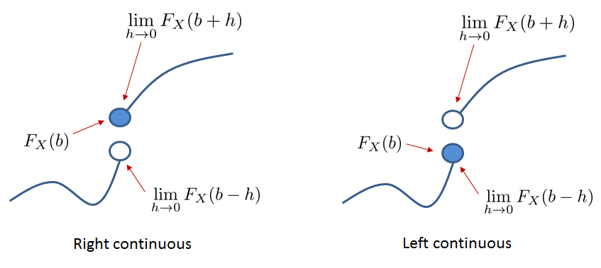
Left-continuous at $x = b$ if $F_X(b) = F_X(b^-) \bydef \lim_{h \rightarrow 0} F_X(b-h)$;
Right-continuous at $x = b$ if $F_X(b) = F_X(b^+) \bydef \lim_{h \rightarrow 0} F_X(b+h)$;
Continuous at $x = b$ if it is both right-continuous and left-continuous at $x =b$. In this case, we have $$\lim_{h \rightarrow 0} F_X(b-h) = \lim_{h \rightarrow 0} F_X(b+h) = F(b).$$

In this definition, the step size $h > 0$ is shrinking to zero. The point $b - h$ stays at the left of $b$, and $b+h$ stays at the right of $b$. Thus, if we set the limit $h \rightarrow 0$, $b-h$ will approach a point $b^-$ whereas $b+h$ will approach a point $b^+$. If it happens that $F_X(b^-) = F_X(b)$ then we say that $F_X$ is left-continuous at $b$. If $F_X(b^+) = F_X(b)$ then we say that $F_X$ is right-continuous at $b$. These are summarized in Figure 4.8.

**Figure 4.8.** The definition of left- and right-continuous at a point $b$.

Whenever $F_X$ has a discontinuous point, it can be left-continuous, right-continuous, or neither. (“Neither” happens if $F_X(b)$ takes a value other than $F_X(b^+)$ or $F_X(b^-)$. You can always create a nasty function that satisfies this condition.) For continuous functions, it is necessary that $F_X(b^-) = F_X(b^+)$. If this happens, there is no gap between the two points.

Theorem 4.3

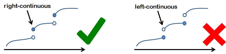
For any random variable $X$ (discrete or continuous), $F_X(x)$ is always right-continuous. That is,

F_X(b) = F_X(b^+) \bydef \lim_{h \rightarrow 0} F_X(b+h)

Right-continuous means that if $F_X(x)$ is piecewise, it must have a solid left end and an empty right end. Figure fig:ch4_continuous_example shows an example of a valid CDF and an invalid CDF.

**Figure 4.9.** A CDF must be right-continuous.

The reason why $F_X$ is always right-continuous is that the inequality $X \le x$ has a closed right-hand limit. Imagine the following situation: A discrete random variable $X$ has four states: $1,2,3,4$. Then,

\begin{aligned} \lim_{h\rightarrow 0} F_X(3+h) = \lim_{h\rightarrow 0} \sum_{k=1}^{\textcolor{black}{\text{``$3+h$''}}}p_X(k) = p_X(1) + p_X(2) + p_X(3) = F_X(3). \end{aligned}

Similarly, if you have a continuous random variable $X$ with a PDF $f_X$, then

\begin{aligned} \lim_{h\rightarrow 0} F_X(b+h) = \lim_{h\rightarrow 0} \int_{-\infty}^{b+h} f_X(t) \;dt = \int_{-\infty}^{b} f_X(t) \;dt = F_X(b). \end{aligned}

In other words, the “$\le$” ensures that the rightmost state is included. If we defined CDF using $<$, we would have gotten left-continuous, but this would be inconvenient because the $<$ requires us to deal with limits whenever we evaluate $X < x$.

Theorem 4.4

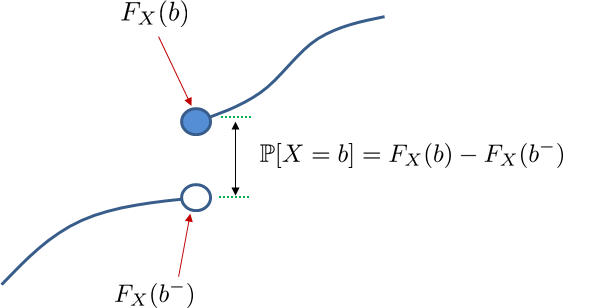
For any random variable $X$ (discrete or continuous), $\Pb[X = b]$ is

\Pb[X = b] = \begin{cases} F_X(b) - F_X(b^-), \quad\mbox{if $F_X$ is discontinuous at $x = b$}\\ 0 , \quad\mbox{otherwise.} \end{cases}

This proposition states that when $F_X(x)$ is discontinuous at $x = b$, then $\Pb[X = b]$ is the difference between $F_X(b)$ and the limit from the left. In other words, the height of the gap determines the probability at the discontinuity. If $F_X(x)$ is continuous at $x = b$, then $F_X(b) = \lim_{h\rightarrow 0} F_X(b-h)$ and so $\Pb[X = b] = 0.$

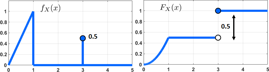
**Figure 4.10.** Illustration of Eq. (4.12). Since the CDF is discontinuous at a point $x = b$, the gap $F_X(b) - F_X(b^-)$ will define the probability $\Pb[X = b]$.

Example 4.15

Consider a random variable $X$ with a PDF

f_X(x) = \begin{cases} x, & 0 \le x \le 1,\\ \frac{1}{2}\delta(x-3), & x = 3,\\ 0, & \text{otherwise}. \end{cases}

The CDF $F_X(x)$ will consist of a few segments. The first segment is $0 \le x < 1$. We can show that

\begin{aligned} F_X(x) = \int_{0}^{x} f_X(t) \;dt = \int_{0}^{x} t \; \;dt = \frac{t^2}{2} \bigg|_{0}^{x} = \frac{x^2}{2}, \quad 0 \le x < 1. \end{aligned}

The second segment is when $1 \le x < 3$. Since there is no new $f_X$ to integrate, the CDF stays at $F_X(x) = F_X(1) = \frac{1}{2}$ for $1 \le x < 3$. The third segment is $x > 3$. Because this range has covered the entire sample space, we have $F_X(x) = 1$ for $x > 3$. How about $x = 3$? We can show that

\begin{aligned} F_X(3) = F_X(3^+) = 1. \end{aligned}

Therefore, to summarize, the CDF is

\begin{aligned} F_X(x) = \begin{cases} 0, &\quad x < 0,\\ \frac{x^2}{2}, &\quad 0 \le x < 1,\\ \frac{1}{2}, &\quad 1 \le x < 3,\\ 1, &\quad x \ge 3. \end{cases} \end{aligned}

A graphical illustration is shown in Figure 4.11.

4.3.3Retrieving PDF from CDF

Thus far, we have only seen how to obtain $F_X(x)$ from $f_X(x)$. In order to go in the reverse direction, we recall the fundamental theorem of calculus. This states that if a function $f$ is continuous, then

f(x) = \frac{d}{\;dx} \int_{a}^{x} f(t) \;dt

for some constant $a$. Using this result for CDF and PDF, we have the following:

Theorem 4.5

The probability density function (PDF) is the derivative of the cumulative distribution function (CDF):

f_X(x) = \frac{d F_X(x)}{\;dx} = \frac{d}{\;dx} \int_{-\infty}^{x} f_X(x') \;dx',

provided $F_X$ is differentiable at $x$. If $F_X$ is not differentiable at $x = x_0$, then,

\begin{aligned} f_X(x) &= \Pb[X = x_0] \delta(x-x_0), \qquad \text{when} \;\; x = x_0. \end{aligned}

Example 4.16

Consider a CDF $$F_X(x) = \begin{cases} 0, & \quad x < 0,\\ 1-\frac{1}{4}e^{-2x}, &\quad x \ge 0. \end{cases}$$ We want to find the PDF $f_X(x)$. To do so, we first show that $F_X(0) = \frac{3}{4}$. This corresponds to a discontinuity at $x = 0$, as shown in Figure 4.12.

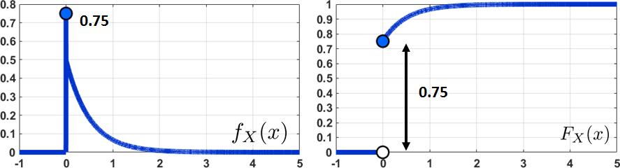
**Figure 4.12.** An example of converting a CDF to a PDF.

Because of the discontinuity, we need to consider three cases:

f_X(x) = \begin{cases} \frac{dF_X(x)}{\;dx}, &\quad x < 0,\\ \Pb[X = 0]\;\delta(x-0), &\quad x = 0,\\ \frac{dF_X(x)}{\;dx}, &\quad x > 0.\\ \end{cases}

When $x < 0$, $F_X(x) = 0$, so $\frac{dF_X(x)}{\;dx} = 0$.

When $x > 0$, $F_X(x) = 1-\frac{1}{4}e^{-2x}$, so $$\frac{dF_X(x)}{dx} = \frac{1}{2}e^{-2x}.$$

When $x = 0$, the probability $\Pb[X = 0]$ is determined by the gap between the solid dot and the empty dot. This yields

\begin{aligned} \Pb[X = 0] &= F_X(0) - \lim_{h \rightarrow 0} F_X(0 - h) \\ &= \frac{3}{4} - 0 = \frac{3}{4}. \end{aligned}

Therefore, the overall PDF is

f_X(x) = \begin{cases} 0, &\quad x < 0,\\ \frac{3}{4}\delta(x-0), &\quad x = 0,\\ \frac{1}{2}e^{-2x}, &\quad x > 0.\\ \end{cases}

Figure 4.12 illustrates this example.

4.3.4CDF: Unifying discrete and continuous random variables

The CDF is always a well-defined function. It is integrable everywhere. If the underlying random variable is continuous, the CDF is also continuous. If the underlying random variable is discrete, the CDF is a staircase function. We have seen enough CDFs for continuous random variables. Let us (re)visit a few discrete random variables.

Example 4.17

(Geometric random variable) Consider a geometric random variable with PMF $p_X(k) = (1-p)^{k-1}p$, for $k = 1,2,\ldots$.

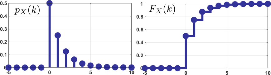
**Figure 4.13.** PMF and CDF of a geometric random variable.

We can show that the CDF is

\begin{aligned} F_X(k) &= \sum_{\ell=1}^{k} p_X(\ell)\\ &= \sum_{\ell=1}^{k} (1-p)^{\ell-1}p \\ &= p \cdot \frac{1-(1-p)^{k}}{1-(1-p)} \\ &= 1-(1-p)^k. \end{aligned}

For a sanity check, we can try to retrieve the PMF from the CDF:

\begin{aligned} p_X(k) &= F_X(k) - F_X(k-1) \\ &= (1-(1-p)^k) - (1-(1-p)^{k-1}) \\ &= (1-p)^{k-1}p. \end{aligned}

A graphical portrayal of this example is shown in Figure 4.13.

If we treat the PMFs as delta functions in the above example, then the continuous definition also applies. Since the CDF is a piecewise constant function, the derivative is exactly a delta function. For some problems, it is easier to start with CDF and then compute the PMF or PDF. Here is an example.

Example 4.18

Let $X_1$, $X_2$ and $X_3$ be three independent discrete uniform random variables with sample space $\Omega = \{1,2,\ldots,10\}$. Define $X = \max\{X_1,X_2,X_3\}$. We want to find the PMF of $X$. To tackle this problem, we first observe that the PMF for $X_1$ is $p_{X_1}(k) = \frac{1}{10}$. Thus, the CDF of $X_1$ is $$F_{X_1}(k) = \sum_{\ell=1}^{k}p_{X_1}(\ell) = \frac{k}{10}.$$ Then, we can show that the CDF of $X$ is

\begin{aligned} F_X(k) = \Pb[X \le k] &= \Pb[\max\{X_1,X_2,X_3\} \le k ]\\ &\overset{(a)}{=} \Pb[X_1 \le k \;\cap X_2 \le k \; \cap X_3 \le k]\\ &\overset{(b)}{=} \Pb[X_1 \le k] \Pb[X_2 \le k] \Pb[X_3 \le k] \\ &= \left(\frac{k}{10}\right)^3, \end{aligned}

where in $(a)$ we use the fact that $\max\{X_1,X_2,X_3\} \le k$ if and only if all three elements are less than $k$, and in $(b)$ we use independence. Consequently, the PMF of $X$ is

p_X(k) = F_X(k) - F_X(k-1) = \left(\frac{k}{10}\right)^3 - \left(\frac{k-1}{10}\right)^3.

What is a CDF?

sep0ex
CDF is $F_X(x) = \Pb[X \le x]$. It is the cumulative sum of the PMF/PDF.
CDF is either a staircase function, a smooth function, or a hybrid. Unlike a PDF, which is not defined for discrete random variables, the CDF is always well defined.
CDF $\overset{\frac{d}{dx}}{\longrightarrow}$ PDF.
CDF $\overset{\int}{\longleftarrow}$ PDF.
Gap of jump in CDF = height of delta in PDF.