Gaussian Random Variables
We now discuss the most important continuous random variable — the Gaussian random variable (also known as the normal random variable). We call it the most important random variable because it is widely used in almost all scientific disciplines. Many of us have used Gaussian random variables before, and perhaps its bell shape is the first lesson we learn in statistics. However, there are many mysteries about Gaussian random variables which you may have missed, such as: Where does the Gaussian random variable come from? Why does it take a bell shape? What are the properties of a Gaussian random variable? The objective of this section is to explain everything you need to know about a Gaussian random variable.
4.6.1Definition of a Gaussian random variable
A Gaussian random variable is a random variable \(X\) such that its PDF is
where \((\mu,\sigma^2)\) are parameters of the distribution. We write $$X \sim \text{Gaussian}(\mu,\sigma^2) \qquad \mbox{or} \qquad X \sim \calN(\mu,\sigma^2)$$ to say that \(X\) is drawn from a Gaussian distribution of parameter \((\mu,\sigma^2)\).
Gaussian random variables have two parameters \((\mu,\sigma^2)\). It is noteworthy that the mean is \(\mu\) and the variance is \(\sigma^2\) — these two parameters are exactly the first moment and the second central moment of the random variable. Most other random variables do not have this property.
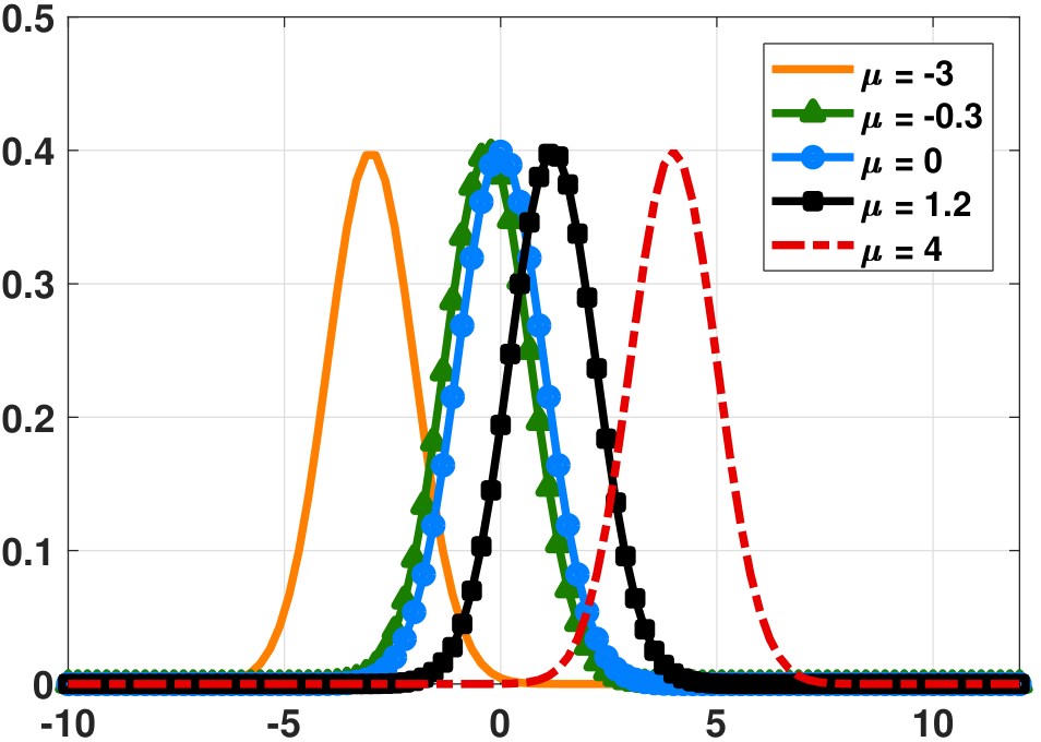
Note that the Gaussian PDF is positive from \(-\infty\) to \(\infty\). Thus, \(f_X(x)\) has a non-zero value for any \(x\), even though the value may be extremely small. A Gaussian random variable is also symmetric about \(\mu\). If \(\mu = 0\), then \(f_X(x)\) is an even function.
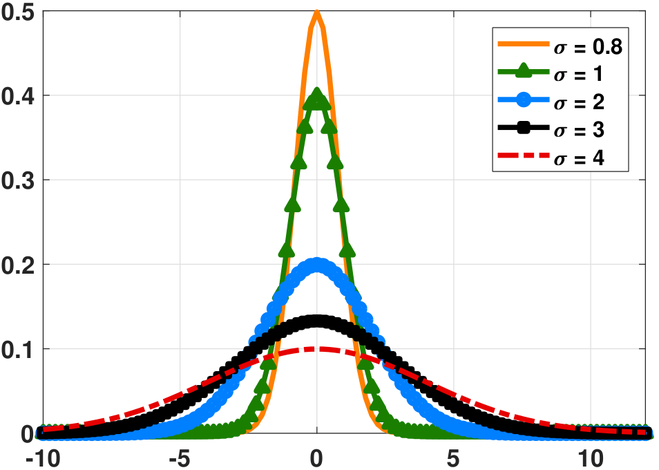
The shape of the Gaussian is illustrated in Figure 4.26. When we fix the variance and change the mean, the PDF of the Gaussian moves left or right depending on the sign of the mean. When we fix the mean and change the variance, the PDF of the Gaussian changes its width. Since any PDF should integrate to unity, a wider Gaussian means that the PDF is shorter. Note also that if \(\sigma\) is very small, it is possible that \(f_X(x) > 1\) although the integration over \(\Omega\) will still be 1.
On a computer, plotting the Gaussian PDF can be done by calling pdf('norm',x) in MATLAB, and stats.norm.pdf in Python.
% MATLAB to generate a Gaussian PDF
    x     = linspace(-10,10,1000);
    mu    = 0; sigma = 1;
    f     = pdf('norm',x,mu,sigma);
plot(x, f);# Python to generate a Gaussian PDF
import numpy as np
import matplotlib.pyplot as plt
import scipy.stats as stats
x = np.linspace(-10,10,1000)
mu = 0; sigma = 1;
f = stats.norm.pdf(x,mu,sigma)
plt.plot(x,f)Our next result concerns the mean and variance of a Gaussian random variable. You may wonder why we need this theorem when we already know that \(\mu\) is the mean and \(\sigma^2\) is the variance. The answer is that we have not proven these two facts.
If \(X \sim \text{Gaussian}(\mu,\sigma^2)\), then
Proof. The expectation can be derived via substitution:
where in (a) we substitute \(y = x - \mu\), in (b) we use the fact that the first integrand is odd so that the integration is 0, and in (c) we observe that integration over the entire sample space of the PDF yields 1.
The variance is also derived by substitution.
where in (a) we substitute \(y = (x-\mu)/\sigma\).
■4.6.2Standard Gaussian
We need to evaluate the probability \(\Pb[a \le X \le b]\) of a Gaussian random variable \(X\) in many practical situations. This involves the integration of the Gaussian PDF, i.e., determining the CDF. Unfortunately, there is no closed-form expression of \(\Pb[a \le X \le b]\) in terms of \((\mu,\sigma^2)\). This leads to what we call the standard Gaussian.
The standard Gaussian (or standard normal) random variable \(X\) has a PDF
That is, \(X \sim \calN(0,1)\) is a Gaussian with \(\mu = 0\) and \(\sigma^2 = 1\).
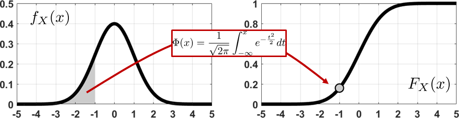
The CDF of the standard Gaussian can be determined by integrating the PDF. We have a special notation for this CDF. Figure 4.27 illustrates the idea.
The CDF of the standard Gaussian is defined as the \(\Phi(\cdot)\) function
% MATLAB code to generate standard Gaussian PDF and CDF
    x = linspace(-5,5,1000);
    f = normpdf(x,0,1);
    F = normcdf(x,0,1);
    figure; plot(x, f);
figure; plot(x, F);# Python code to generate standard Gaussian PDF and CDF
import numpy as np
import matplotlib.pyplot as plt
import scipy.stats as stats
x = np.linspace(-10,10,1000)
f = stats.norm.pdf(x)
F = stats.norm.cdf(x)
plt.plot(x,f); plt.show()
plt.plot(x,F); plt.show()The standard Gaussian's CDF is related to a so-called error function defined as
It is easy to link \(\Phi(x)\) with \(\text{erf}(x)\):
With the standard Gaussian CDF, we can define the CDF of an arbitrary Gaussian.
Let \(X \sim \calN(\mu,\sigma^2)\). Then
Proof. We start by expressing \(F_X(x)\):
Substituting \(y = \frac{t-\mu}{\sigma}\), and using the definition of standard Gaussian, we have
If you would like to verify this on a computer, you can try the following code.
% MATLAB code to verify standardized Gaussian
    x = linspace(-5,5,1000);
    mu = 3; sigma = 2;
    f1 = normpdf((x-mu)/sigma,0,1); % standardized
f2 = normpdf(x, mu, sigma); % raw# Python code to verify standardized Gaussian
import numpy as np
import matplotlib.pyplot as plt
import scipy.stats as stats
x = np.linspace(-5,5,1000)
mu = 3; sigma = 2;
f1 = stats.norm.pdf((x-mu)/sigma,0,1) # standardized
f2 = stats.norm.cdf(x,mu,sigma) # rawAn immediate consequence of this result is that
To see this, note that
The inequality signs of the two end points are not important. That is, the statement also holds for \(\Pb[a \le X \le b]\) or \(\Pb[a < X < b]\), because \(X\) is a continuous random variable at every \(x\). Thus, \(\Pb[X = a] = \Pb[X = b] = 0\) for any \(a\) and \(b\). Besides this, \(\Phi\) has several properties of interest. See if you can prove these:
Let \(X \sim \calN(\mu,\sigma^2)\). Then the following results hold:
- sep0ex
- \(\Phi(y) = 1-\Phi(-y)\).
- \(\Pb[X \ge b] = 1 - \Phi\left(\frac{b-\mu}{\sigma}\right)\).
- \(\Pb[|X| \ge b] = 1 - \Phi\left(\frac{b-\mu}{\sigma}\right) + \Phi\left(\frac{-b-\mu}{\sigma}\right)\).
4.6.3Skewness and kurtosis
In modern data analysis we are sometimes interested in high-order moments. Here we consider two useful quantities: skewness and kurtosis.
For a random variable \(X\) with PDF \(f_X(x)\), define the following central moments as
As you can see from the definitions above, skewness is the third central moment, whereas kurtosis is the fourth central moment. Both skewness and kurtosis can be regarded as “deviations” from a standard Gaussian not in terms of mean and variance but in terms of shape.
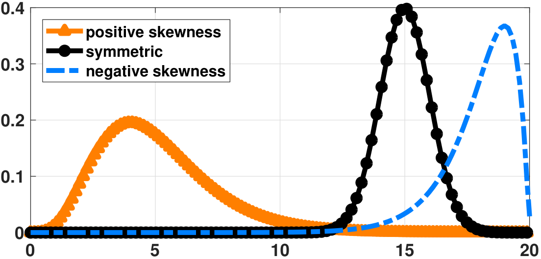
Skewness measures the asymmetry of the distribution. Figure 4.28 shows three different distributions: one with left skewness, one with right skewness, and one symmetric. The skewness of a curve is
- sep0em
- Skewed towards left: negative
- Skewed towards right: positive
- Symmetric: zero
- sep0ex
- \(\E\left[\left(\frac{X-\mu}{\sigma}\right)^3\right]\).
- Measures the asymmetry of the distribution.
- Gaussian has skewness 0.
Kurtosis measures how heavy-tailed the distribution is. There are two forms of kurtosis: one is the standard kurtosis, which is the fourth central moment, and the other is the excess kurtosis, which is \(\kappa_{\text{excess}} = \kappa - 3\). The constant 3 comes from the kurtosis of a standard Gaussian. Excess kurtosis is more widely used in data analysis. The interpretation of kurtosis is the comparison to a Gaussian. If the excess kurtosis is positive, the distribution has a tail that decays more slowly than a Gaussian. If the excess kurtosis is negative, the distribution has a tail that decays faster than a Gaussian. Figure 4.29 illustrates the (excess) kurtosis of three different distributions.
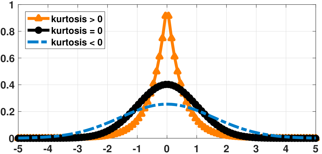
- sep0ex
- \(\kappa = \E\left[\left(\frac{X-\mu}{\sigma}\right)^4\right]\).
- Measures how heavy-tailed the distribution is. Gaussian has kurtosis 3.
- Some statisticians prefer excess kurtosis \(\kappa-3\), so that Gaussian has excess kurtosis 0.
| Random variable | Mean | Variance | Skewness | Excess kurtosis |
| \(\mu\) | \(\sigma^2\) | \(\gamma\) | \(\kappa - 3\) | |
| lightgray Bernoulli | \(p\) | \(p(1-p)\) | \(\frac{1-2p}{\sqrt{p(1-p)}}\) | \(\frac{1}{1-p} + \frac{1}{p} - 6\) |
| Binomial | \(np\) | \(np(1-p)\) | \(\frac{1-2p}{\sqrt{np(1-p)}}\) | \(\frac{6p^2-6p+1}{np(1-p)}\) |
| lightgray Geometric | \(\frac{1}{p}\) | \(\frac{1-p}{p^2}\) | \(\frac{2-p}{\sqrt{1-p}}\) | \(\frac{p^2-6p+6}{1-p}\) |
| Poisson | \(\lambda\) | \(\lambda\) | \(\frac{1}{\sqrt{\lambda}}\) | \(\frac{1}{\lambda}\) |
| lightgray Uniform | \(\frac{a+b}{2}\) | \(\frac{(b-a)^2}{12}\) | 0 | \(-\frac{6}{5}\) |
| Exponential | \(\frac{1}{\lambda}\) | \(\frac{1}{\lambda^2}\) | 2 | 6 |
| lightgray Gaussian | \(\mu\) | \(\sigma^2\) | 0 | \(0\) |
On a computer, computing the empirical skewness and kurtosis is done by built-in commands. Their implementations are based on the finite-sample calculations
The MATLAB and Python built-in commands are shown below, using a gamma distribution as an example.
% MATLAB code to compute skewness and kurtosis
    X = random('gamma',3,5,[10000,1]);
    s = skewness(X);
k = kurtosis(X);# Python code to compute skewness and kurtosis
import scipy.stats as stats
X = stats.gamma.rvs(3,5,size=10000)
s = stats.skew(X)
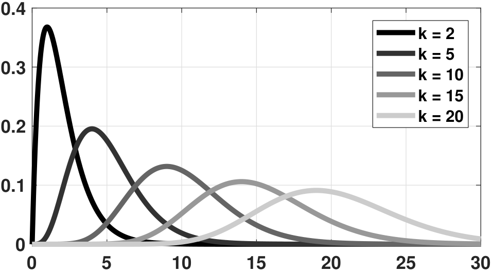
k = stats.kurtosis(X)To further illustrate the behavior of skewness and kurtosis, we consider an example using the gamma random variable \(X\). The PDF of \(X\) is given by the equation
where \(\Gamma(\cdot)\) is known as the gamma function. If \(k\) is an integer, the gamma function is just the factorial: \(\Gamma(k) = (k-1)!\). A gamma random variable is parametrized by two parameters \((k,\theta)\). As \(k\) increases or decreases, the shape of the PDF will change. For example, when \(k = 1\), the distribution is simplified to an exponential distribution.
Without going through the (tedious) integration, we can show that the skewness and the (excess) kurtosis of \(\text{Gamma}(k,\theta)\) are
As we can see from these results, the skewness and kurtosis diminish as \(k\) grows. This can be confirmed from the PDF of \(\text{Gamma}(k,\theta)\) as shown in Figure 4.30.
Let us look at a real example. On April 15, 1912, RMS Titanic sank after hitting an iceberg. The disaster killed 1502 out of 2224 passengers and crew. A hundred years later, we want to analyze the data. At https://www.kaggle.com/c/titanic/ there is a dataset collecting the identities, age, gender, etc., of the passengers. We partition the dataset into two: one for those who died and the other one for those who survived. We plot the histograms of the ages of the two groups and compute several statistics of the dataset. Figure 4.31 shows the two datasets.
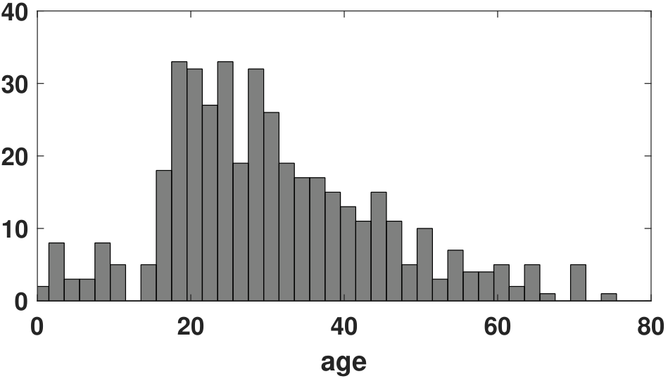
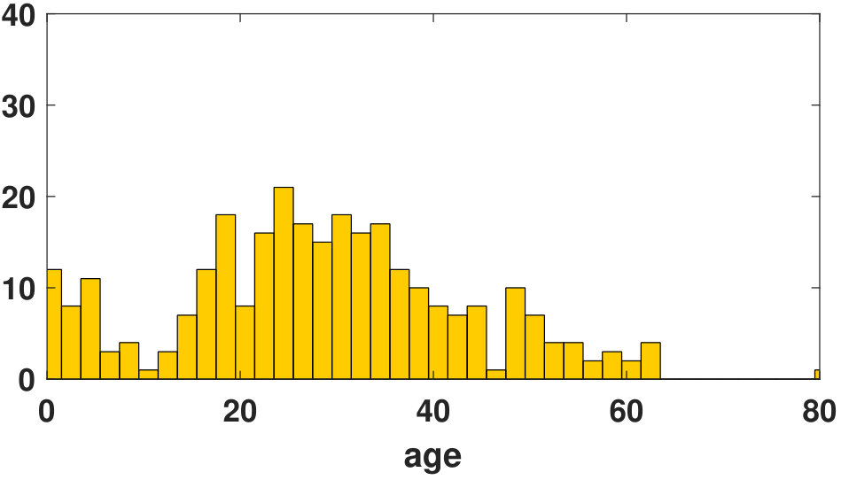
| Statistics | Group 1 (Died) | Group 2 (Survived) |
| Mean | 30.6262 | 28.3437 |
| Standard Deviation | 14.1721 | 14.9510 |
| Skewness | 0.5835 | 0.1795 |
| Excess Kurtosis | 0.2652 | \(-0.0772\) |
Note that the two groups of people have very similar means and standard deviations. In other words, if we only compare the mean and standard deviation, it is nearly impossible to differentiate the two groups. However, the skewness and kurtosis provide more information related to the shape of the histograms. For example, Group 1 has more positive skewness, whereas Group 2 is almost symmetrical. One interpretation is that more young people offered lifeboats to children and older people. The kurtosis of Group 1 is slightly positive, whereas that of Group 2 is slightly negative. Therefore, high-order moments can sometimes be useful for data analysis.
4.6.4Origin of Gaussian random variables
The Gaussian random variable has a long history. Here, we provide one perspective on why Gaussian random variables are so useful. We give some intuitive arguments but leave the formal mathematical treatment for later when we introduce the Central Limit Theorem.
Let's begin with a numerical experiment. Consider throwing a fair die. We know that this will give us a (discrete) uniform random variable \(X\). If we repeat the experiment many times, we can plot the histogram, and it will return us a plot of 6 impulses with equal height, as shown in Figure 4.32(a).
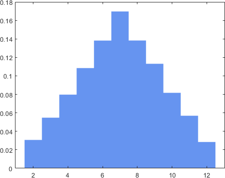
Now, suppose we throw two dice. Call them \(X_1\) and \(X_2\), and let \(Z = X_1 + X_2\), i.e., the sum of two dice. We want to find the distribution of \(Z\). To do so, we first list out all the possible outcomes in the sample space; this gives us \(\{(1,1),(1,2),\ldots,(6,6)\}\). We then sum the numbers, which gives us a list of states of \(Z\): \(\{2,3,4,\ldots,12\}\). The probability of getting these states is shown in Figure 4.32(b), which has a triangular shape. The triangular shape makes sense because to get the state “2”, we must have the pair \((1,1)\), which is quite unlikely. However, if we want to get the state 7, it would be much easier to get a pair, e.g., \((6,1),(5,2),(4,3),(3,4),(2,5),(1,6)\) would all do the job.
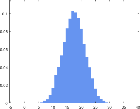
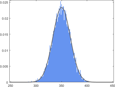
Now, what will happen if we throw 5 dice and consider \(Z = X_1 + X_2 + \cdots + X_{5}\)? It turns out that the distribution will continue to evolve and give something like Figure 4.32(c). This is starting to approximate a bell shape. Finally, if we throw 100 dice and consider \(Z = X_1 + X_2 + \cdots + X_{100}\), the distribution will look like Figure 4.32(d). The shape is becoming a Gaussian! This numerical example demonstrates a fascinating phenomenon: As we sum more random variables, the distribution of the sum will converge to a Gaussian.
If you are curious about how we plot the above figures, the following MATLAB and Python code can be useful.
% MATLAB code to show the histogram of Z = X1+X2+X3
    N  = 10000;
    X1 = randi(6,1,N);
    X2 = randi(6,1,N);
    X3 = randi(6,1,N);
    Z  = X1 + X2 + X3;
histogram(Z, 2.5:18.5);# Python code to show the histogram of Z = X1+X2+X3
import numpy as np
import matplotlib.pyplot as plt
N = 10000
X1 = np.random.randint(1,6,size=N)
X2 = np.random.randint(1,6,size=N)
X3 = np.random.randint(1,6,size=N)
Z = X1 + X2 + X3
plt.hist(Z,bins=np.arange(2.5,18.5))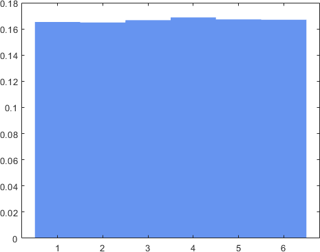
Can we provide a more formal description of this? Yes, but we need some new mathematical tools that we have not yet developed. So, for the time being, we will outline the flow of the arguments and leave the technical details to a later chapter. Suppose we have two independent random variables with identical distributions, e.g., \(X_1\) and \(X_2\), where both are uniform. This gives us PDFs \(f_{X_1}(x)\) and \(f_{X_2}(x)\) that are two identical rectangular functions. By what operation can we combine these two rectangular functions and create a triangle function? The key lies in the concept of convolution. If you convolve two rectangle functions, you will get a triangle function. Here we define the convolution of \(f_X\) as
In fact, for any pair of random variables \(X_1\) and \(X_2\) (not necessarily uniform random variables), the sum \(Z = X_1+X_2\) will have a PDF given by the convolution of the two PDFs. We have not yet proven this, but if you trust what we are saying, we can effectively generalize this argument to many random variables. If we have \(N\) random variables, then the sum \(Z = X_1 + X_2 + \cdots + X_N\) will have a PDF that is the result of \(N\) convolutions of all the individual PDFs.
- sep0ex
- Summing \(X+Y\) is equivalent to convolving the PDFs \(f_X \ast f_Y\).
- If you sum many random variables, you convolve all their PDFs.
How do we analyze these convolutions? We need a second set of tools related to Fourier transforms. The Fourier transform of a PDF is known as the characteristic function, which we will discuss later, but the name is not important now. What matters is the important property of the Fourier transform, that a convolution in the original space is multiplication in the Fourier space. That is,
Multiplication in the Fourier space is much easier to analyze. In particular, for independent and identically distributed random variables, the multiplication will easily translate to addition in the exponent. Then, by truncating the exponent to the second order, we can show that the limiting object in the Fourier space is approaching a Gaussian. Finally, since the inverse Fourier transform of a Gaussian remains a Gaussian, we have shown that the infinite convolution will give us a Gaussian.
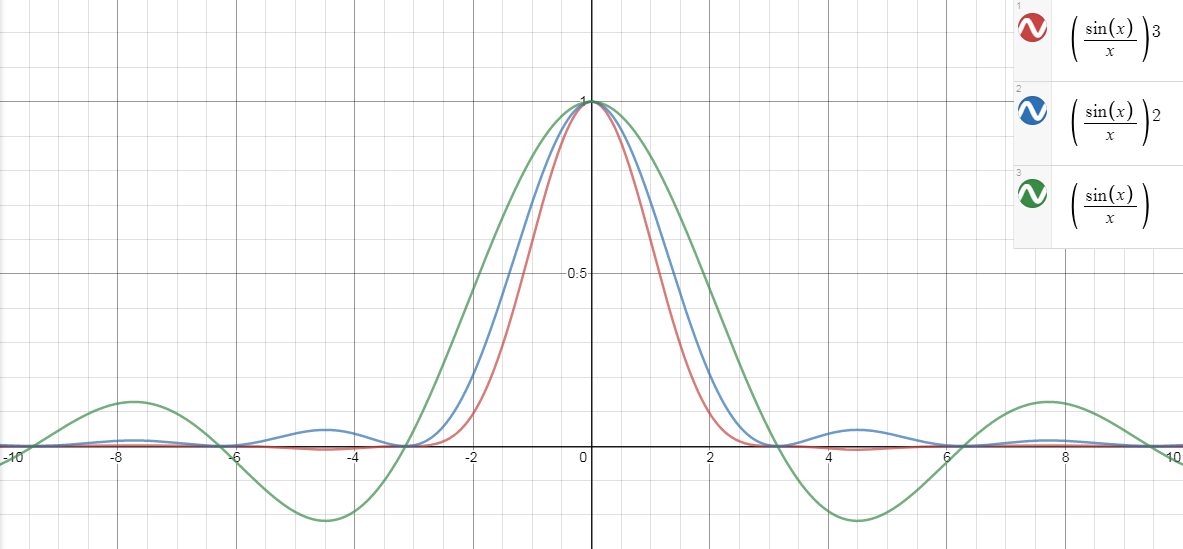
Here is some numerical evidence for what we have just described. Recall that the Fourier transform of a rectangle function is the sinc function. Therefore, if we have an infinite convolution of rectangular functions, equivalently, we have an infinite product of sinc functions in the Fourier space. Multiplying sinc functions is reasonably easy. See Figure 4.33 for the first three sincs. It is evident that with just three sinc functions, the shape closely approximates a Gaussian.
How about distributions that are not rectangular? We invite you to numerically visualize the effect when you convolve the function many times. You will see that as the number of convolutions grows, the resulting function will become more and more like a Gaussian. Regardless of what the input random variables are, as long as you add them, the sum will have a distribution that looks like a Gaussian:
We use the notation \(\rightsquigarrow\) to emphasize that the convergence is not the usual form of convergence. We will make this precise later.
The implication of this line of discussion is important. Regardless of the underlying true physical process, if we are only interested in the sum (or average), the distribution will be more or less Gaussian. In most engineering problems, we are looking at the sum or average. For example, when generating an image using an image sensor, the sensor will add a certain amount of read noise. Read noise is caused by the random fluctuation of the electrons in the transistors due to thermal distortions. For high-photon-flux situations, we are typically interested in the average read noise rather than the electron-level read noise. Thus Gaussian random variables become a reasonable model for that. In other applications, such as imaging through a turbulent medium, the random phase distortions (which alter the phase of the wavefront) can also be modeled as a Gaussian random variable. Here is the summary of the origin of a Gaussian random variable:
- sep0ex
- When we sum many independent random variables, the resulting random variable is a Gaussian.
- This is known as the Central Limit Theorem. The theorem applies to any random variable.
- Summing random variables is equivalent to convolving the PDFs. Convolving PDFs infinitely many times yields the bell shape.