eBook › Chapter 4 · Continuous Random Variables

Section 4.5

Uniform and Exponential Random Variables

There are many useful continuous random variables. In this section, we discuss two of them: uniform random variables and exponential random variables. In the next section, we will discuss the Gaussian random variables. Similarly to the way we discussed discrete random variables, we take a generative / synthesis perspective when studying continuous random variables. We assume we have access to the PDF of the random variables so we can derive the theoretical mean and variance. The opposite direction, namely inferring the underlying model parameters from a dataset, will be discussed later.

4.5.1Uniform random variables

Definition 4.11

Let $X$ be a continuous uniform random variable. The PDF of $X$ is

f_X(x) = \begin{cases} \frac{1}{b-a}, & \quad a \le x \le b, \\ 0 , & \quad \mbox{otherwise}, \end{cases}

where $[a,b]$ is the interval on which $X$ is defined. We write $$X \sim \mathrm{Uniform}(a,b)$$ to mean that $X$ is drawn from a uniform distribution on an interval $[a,b]$.

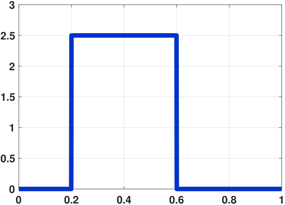
The shape of the PDF of a uniform random variable is shown in Figure 4.19. In this figure, we assume that the random variables $X \sim \text{Uniform}(0.2,0.6)$ are taken from the sample space $\Omega = [0,1]$. Note that the height of the uniform distribution is greater than 1, since

f_X(x) = \begin{cases} \frac{1}{0.6-0.2} = 2.5, & \quad 0.2 \le x \le 0.6, \\ 0 , & \quad \mbox{otherwise}. \end{cases}

There is nothing wrong with this PDF, because $f_X(x)$ is the probability per unit length. If we integrate $f_X(x)$ over any sub-interval between 0.2 and 0.6, we can show that the probability is between 0 and 1.

**Figure 4.19.** The PDF and CDF of $X \sim \text{Uniform}(0.2,0.6)$.

The CDF of a uniform random variable can be determined by integrating $f_X(x)$:

\begin{aligned} F_X(x) &= \int_{-\infty}^x f_X(t) \;dt\\ &=\int_{a}^{x} \frac{1}{b-a} \;dt \\ &= \frac{x-a}{b-a}, \qquad\qquad\qquad a \le x \le b. \end{aligned}

Therefore, the complete CDF is

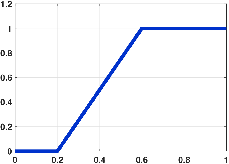
F_X(x) = \begin{cases} 0, &\quad x < a,\\ \frac{x-a}{b-a}, &\quad a \le x \le b,\\ 1, &\quad x > b. \end{cases}

The corresponding CDF for the PDF we showed in Figure 4.19(a) is shown in Figure 4.19(b). It can be seen that although the height of the PDF exceeds 1, the CDF grows linearly and saturates at 1.

Remark. The uniform distribution can also be defined for discrete random variables. In this case, the probability mass function is given by $$p_X(k) = \frac{1}{b - a + 1}, \quad k = a, {a + 1}, \ldots, b.$$ The presence of “1” in the denominator of the PMF is because $k$ runs from $a$ to $b$, including the two endpoints.

In MATLAB and Python, generating uniform random numbers can be done by calling commands unifrnd (MATLAB), and stats.uniform.rvs (Python). For discrete uniform random variables, in MATLAB the command is unidrnd, and in Python the command is stats.randint.

MATLAB

% MATLAB code to generate 1000 uniform random numbers
    a = 0; b = 1;
    X = unifrnd(a,b,[1000,1]);
    hist(X);

Python

# Python code to generate 1000 uniform random numbers
    import scipy.stats as stats
    a = 0; b = 1;
    X = stats.uniform.rvs(a,b,size=1000)
    plt.hist(X);

To compute the empirical average and variance of the random numbers in MATLAB we can call the command mean and var. The corresponding command in Python is np.mean and np.var. We can also compute the median and mode, as shown below.

MATLAB

% MATLAB code to compute empirical mean, var, median, mode
    X = unifrnd(a,b,[1000,1]);
    M = mean(X);
    V = var(X);
    Med = median(X);
    Mod = mode(X);

Python

# Python code to compute empirical mean, var, median, mode
    X = stats.uniform.rvs(a,b,size=1000)
    M = np.mean(X)
    V = np.var(X)
    Med = np.median(X)
    Mod = stats.mode(X)

The mean and variance of a uniform random variable are given by the theorem below.

Theorem 4.8

If $X \sim \mathrm{Uniform}(a,b)$, then

\begin{aligned} \E[X] &= \frac{a+b}{2} \quad\mbox{and}\quad \Var[X] = \frac{(b-a)^2}{12}. \end{aligned}

Proof. We have derived these results before. Here is a recap for completeness:

\begin{aligned} \E[X] &= \int_{-\infty}^{\infty} x f_X(x) \;dx = \int_{a}^{b} \frac{x}{b-a} \;dx = \frac{a+b}{2},\\ \E[X^2] &= \int_{-\infty}^{\infty} x^2 f_X(x) \;dx = \int_{a}^{b} \frac{x^2}{b-a} \;dx = \frac{a^2+ab+b^2}{3},\\ \Var[X] &= \E[X^2] - \E[X]^2 = \frac{(b-a)^2}{12}. \end{aligned}

■

The result should be intuitive because it says that the mean is the midpoint of the PDF.

When will we encounter a uniform random variable? Uniform random variables are one of the most elementary continuous random variables. Given a uniform random variable, we can construct any random variable by using an appropriate transformation. We will discuss this technique as part of our discussion about generating random numbers.

In MATLAB, computing the mean and variance of a uniform random variable can be done using the command unifstat. The Python command is stats.uniform.stats.

MATLAB

% MATLAB code to compute mean and variance
    a = 0; b = 1;
    [M,V] = unifstat(a,b)

Python

# Python code to compute mean and variance
    import scipy.stats as stats
    a = 0; b = 1;
    M, V = stats.uniform.stats(a,b,moments='mv')

To evaluate the probability $\Pb[\ell \le X \le u]$ for a uniform random variable, we can call unifcdf in MATLAB and stats.uniform.cdf in Python

MATLAB

% MATLAB code to compute the probability P(0.2 < X < 0.3)
    a = 0; b = 1;
    F = unifcdf(0.3,a,b) - unifcdf(0.2,a,b)

Python

# Python code to compute the probability P(0.2 < X < 0.3)
    a = 0; b = 1;
    F = stats.uniform.cdf(0.3,a,b)-stats.uniform.cdf(0.2,a,b)

An alternative is to define an object rv = stats.uniform, and call the CDF attribute:

Python

# Python code to compute the probability P(0.2 < X < 0.3)
    a = 0; b = 1;
    rv = stats.uniform(a,b)
    F = rv.cdf(0.3)-rv.cdf(0.2)

4.5.2Exponential random variables

Definition 4.12

Let $X$ be an exponential random variable. The PDF of $X$ is

f_X(x) = \begin{cases} \lambda e^{-\lambda x}, & \quad x \ge 0, \\ 0 , & \quad \mbox{otherwise}, \end{cases}

where $\lambda > 0$ is a parameter. We write $$X \sim \mathrm{Exponential}(\lambda)$$ to mean that $X$ is drawn from an exponential distribution of parameter $\lambda$.

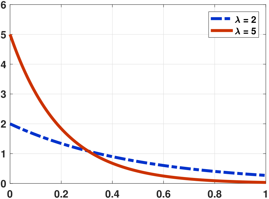
In this definition, the parameter $\lambda$ of the exponential random variable determines the rate of decay. A large $\lambda$ implies a faster decay. The PDF of an exponential random variable is illustrated in Figure 4.20. We show two values of $\lambda$. Note that the initial value $f_X(0)$ is

f_X(0) = \lambda e^{-\lambda 0} = \lambda.

Therefore, as long as $\lambda > 1$, $f_X(0)$ will exceed 1.

**Figure 4.20.** (a) The PDF and (b) the CDF of $X \sim \text{Exponential}(\lambda)$.

The CDF of an exponential random variable can be determined by

\begin{aligned} F_X(x) &= \int_{-\infty}^{x} f_X(t) \;dt \\ &= \int_0^{x} \lambda e^{-\lambda t} \;dt = 1-e^{-\lambda x}, \qquad\qquad x \ge 0. \end{aligned}

Therefore, if we consider the entire real line, the CDF is

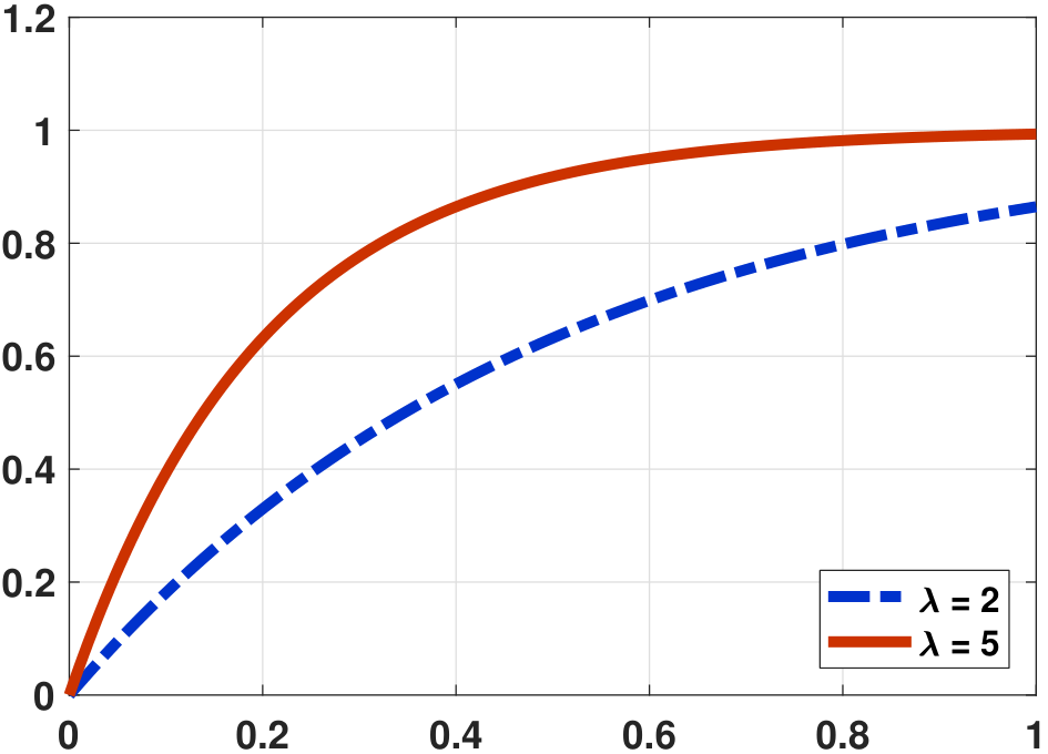
F_X(x) = \begin{cases} 0, &\quad x < 0,\\ 1-e^{-\lambda x}, &\quad x \ge 0. \end{cases}

The corresponding CDFs for the PDFs shown in Figure 4.20(a) are shown in Figure 4.20(b). For larger $\lambda$, the PDF $f_X(x)$ decays faster but the CDF $F_X(x)$ increases faster.

In MATLAB, the code used to generate Figure 4.20(a) is shown below. There are multiple ways of doing this. An alternative way is to call exppdf, which will return the same result. In Python, the corresponding command is stats.expon.pdf. Note that in Python the parameter $\lambda$ is specified in scale option.

MATLAB

% MATLAB code to plot the exponential PDF
    lambda1 = 1/2;  lambda2 = 1/5;
    x = linspace(0,1,1000);
    f1 = pdf('exp',x, lambda1);
    f2 = pdf('exp',x, lambda2);
    plot(x, f1, 'LineWidth', 4, 'Color', [0 0.2 0.8]); hold on;
    plot(x, f2, 'LineWidth', 4, 'Color', [0.8 0.2 0]);

Python

# Python code to plot the exponential PDF
    lambd1 = 1/2
    lambd2 = 1/5
    x = np.linspace(0,1,1000)
    f1 = stats.expon.pdf(x,scale=lambd1)
    f2 = stats.expon.pdf(x,scale=lambd2)
    plt.plot(x, f1)
    plt.plot(x, f2)

To plot the CDF, we replace pdf by cdf. Similarly, in Python we replace expon.pdf by expon.cdf.

MATLAB

% MATLAB code to plot the exponential CDF
    F = cdf('exp',x, lambda1);
    plot(x, F, 'LineWidth', 4, 'Color', [0 0.2 0.8]);

Python

# Python code to plot the exponential CDF
    F = stats.expon.cdf(x,scale=lambd1)
    plt.plot(x, F)

Theorem 4.9

If $X \sim \mathrm{Exponential}(\lambda)$, then

\begin{aligned} \E[X] &= \frac{1}{\lambda} \quad\mbox{and}\quad \Var[X] = \frac{1}{\lambda^2}. \end{aligned}

Proof. We have discussed this proof before. Here is a recap for completeness:

\begin{aligned} \E[X] = \int_{-\infty}^{\infty} x f_X(x) \;dx &= \int_{0}^{\infty} \lambda x e^{-\lambda x} \;dx \\ &= -\int_{0}^{\infty} x d e^{-\lambda x} \\ &= -x e^{-\lambda x} \Big|_{0}^{\infty} + \int_0^{\infty} e^{-\lambda x}\;dx = \frac{1}{\lambda}, \end{aligned}

\begin{aligned} \E[X^2] = \int_{-\infty}^{\infty} x^2 f_X(x) \;dx &= \int_{0}^{\infty} \lambda x^2 e^{-\lambda x} \;dx \\ &= -\int_{0}^{\infty} x^2 d e^{-\lambda x} \\ &= -x^2 e^{-\lambda x} \Big|_{0}^{\infty} + \int_0^{\infty} 2x e^{-\lambda x}\;dx \\ &= 0 + \frac{2}{\lambda}\E[X] = \frac{2}{\lambda^2}. \end{aligned}

Thus, $\Var[X] = \E[X^2] - \E[X]^2 = \frac{1}{\lambda^2}$.

■

Computing the mean and variance of an exponential random variable in MATLAB and Python follows similar procedures to those described above.

4.5.3Origin of exponential random variables

Exponential random variables are closely related to Poisson random variables. Recall that the definition of a Poisson random variable is a random variable that describes the number of events that happen in a certain period, e.g., photon arrivals, number of pedestrians, phone calls, etc. We summarize the origin of an exponential random variable as follows.

What is the origin of exponential random variables?

sep0ex
An exponential random variable is the interarrival time between two consecutive Poisson events.
That is, an exponential random variable is how much time it takes to go from $N$ Poisson counts to $N+1$ Poisson counts.

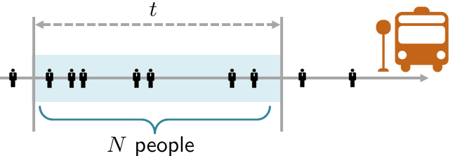
An example will clarify this concept. Imagine that you are waiting for a bus, as illustrated in Figure 4.21. Passengers arrive at the bus stop with an arrival rate $\lambda$ per unit time. Thus, for some time $t$, the average number of people that arrive is $\lambda t$. Let $N$ be a random variable denoting the number of people. We assume that $N$ is Poisson with a parameter $\lambda t$. That is, for any duration $t$, the probability of observing $n$ people follows the PMF

\Pb[N = n] = \frac{(\lambda t)^n}{n!}e^{-\lambda t}.

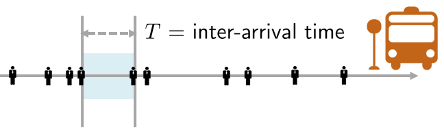
Let $T$ be the interarrival time between two people, by which we mean the time between two consecutive arrivals, as shown in Figure 4.22. Note that $T$ is a random variable because $T$ depends on $N$, which is itself a random variable. To find the PDF of $T$, we first find the CDF of $T$. We note that

\begin{aligned} \Pb[T > t] &\overset{(a)}{=} \Pb[\mbox{interarrival time } > t] \\ &\overset{(b)}{=} \Pb[\mbox{no arrival in } t] \overset{(c)}{=} \Pb[N = 0] = \frac{(\lambda t)^0}{0!}e^{-\lambda t} = e^{-\lambda t}. \end{aligned}

In this set of arguments, (a) holds because $T$ is the interarrival time, and (b) holds because interarrival time is between two consecutive arrivals. If the interarrival time is larger than $t$, there is no arrival during the period. Equality (c) holds because $N$ is the number of passengers.

**Figure 4.22.** The interarrival time $T$ between two consecutive Poisson events is an exponential random variable.

Since $\Pb[T > t] = 1 - F_T(t)$, where $F_T(t)$ is the CDF of $T$, we can show that

\begin{aligned} F_T(t) &= 1-e^{-\lambda t}, \\ f_T(t) &= \frac{d}{dt} F_T(t) = \lambda e^{-\lambda t}. \end{aligned}

Therefore, the interarrival time $T$ follows an exponential distribution.

Since exponential random variables are tightly connected to Poisson random variables, we should expect them to be useful for modeling temporal events. We discuss two examples.

4.5.4Applications of exponential random variables

Example 4.22

(Photon arrivals) Single-photon image sensors are designed to operate in the photon-limited regime. The number-one goal of using these sensors is to count the number of arriving photons precisely. However, for some applications not all single-photon image sensors are used to count photons. Some are used to measure the time between two photon arrivals, such as time-of-flight systems. In this case, we are interested in measuring the time it takes for a pulse to bounce back to the sensor. The more time it takes for a pulse to come back, the greater the distance between the object and the sensor. Other applications utilize the time information. For example, high-dynamic-range imaging can be achieved by recording the time between two photon arrivals because brighter regions have a higher Poisson rate $\lambda$ and darker regions have a lower $\lambda$.

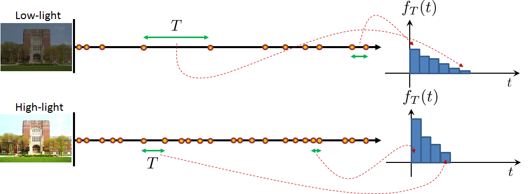
The figure above illustrates an example of high-dynamic-range imaging. When the scene is bright, the large $\lambda$ will generate more photons. Therefore, the interarrival time between the consecutive photons will be relatively short. If we plot the histogram of the interarrival time, we observe that most of the interarrival time will be concentrated at small values. Dark regions behave in the opposite manner. The interarrival time will typically be much longer. In addition, because there is more variation in the photon arrival times, the histogram will look shorter and wider. Nevertheless, both cases are modeled by the exponential random variable.

Example 4.23

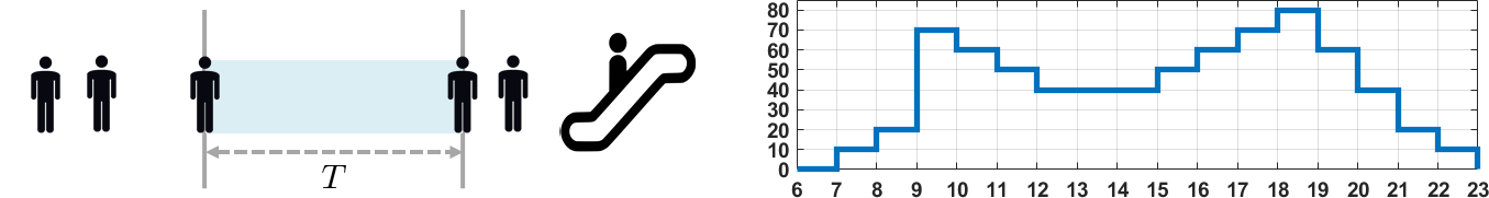
(Energy-efficient escalator) Many airports today have installed variable-speed escalators. These escalators change their speeds according to the traffic. If there are no passengers for more than a certain period (say, 60 seconds), the escalator will switch from the full-speed mode to the low-speed mode. For moderately busy escalators, the variable-speed configuration can save energy. The interesting data-science problem is to determine, given a traffic pattern, e.g., the one shown in Figure 4.24, whether we can predict the amount of energy savings.

We will not dive into the details of this problem, but we can briefly discuss the principle. Consider a fixed arrival rate $\lambda$ (say, the average from 07:00 to 08:00). The interarrival time, according to our discussion above, follows an exponential distribution. So we know that

f_T(t) = \lambda e^{-\lambda t}.

Suppose that the escalator switches to low-speed mode when the interarrival time exceeds $\tau$. Then we can define a new variable $Y$ to denote the amount of time that the escalator will operate in the low-speed mode. This new variable is

\begin{aligned} Y = \begin{cases} T - \tau, &\qquad T > \tau,\\ 0, &\qquad T \le \tau. \end{cases} \end{aligned}

In other words, if the interarrival time $T$ is more than $\tau$, then the amount of time saved $Y$ takes the value $T - \tau$, but if the interarrival time is less than $\tau$, then there is no saving.

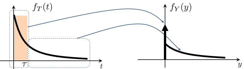
**Figure 4.24.** The variable-speed escalator problem. [Left] We model the passengers as independent Poisson arrivals. Thus, the interarrival time is exponential. [Right] A hypothetical passenger arrival rate (number of people per minute), from 06:00 to 23:00.

The PDF of $Y$ can be computed according to Figure 4.25. There are two parts to the calculation. When $Y = 0$, there is a probability mass such that

\begin{aligned} f_Y(0) = \Pb[Y = 0] &= \int_{0}^{\tau} f_T(t)\;dt = \int_0^\tau \lambda e^{-\lambda t}\;dt = 1-e^{-\lambda \tau}. \end{aligned}

For other values of $y$, we can show that

\begin{aligned} f_Y(y) = f_T(y+\tau) = \lambda e^{-\lambda (y+\tau)}. \end{aligned}

Therefore, to summarize, we can show that the PDF of $Y$ is

\begin{aligned} f_Y(y) = \begin{cases} (1-e^{-\lambda \tau})\delta(y), &\qquad y = 0,\\ \lambda e^{-\lambda (y+\tau)}, &\qquad y > 0. \end{cases} \end{aligned}

Consequently, we can compute $\E[Y]$ and $\Var[Y]$ and analyze how these values change with $\lambda$ (which itself changes with the time of day). Furthermore, we can analyze the amount of savings in terms of dollars. We leave these problems as an exercise.

Closing remark. The photon arrival problem and the escalator problem are two of many examples we can find in which exponential random variables are useful for modeling a problem. We did not go into the details of the problems because each of them requires some additional modeling to address the real practical problem. We encourage you to explore these problems further. Our message is simple: Many problems can be modeled by exponential random variables, most of which are associated with time.