Median, Mode, and Mean
There are three statistical quantities that we are frequently interested in: mean, mode, and median. We all know how to compute these from a dataset. For example, to compute the median of a dataset, we sort the data and pick the number that sits in the 50th percentile. However, the median computed in this way is the empirical median, i.e., it is a value computed from a particular dataset. If the data is generated from a random variable (with a given PDF), how do we compute the mean, median, and mode?
4.4.1Median
Imagine you have a sequence of numbers as shown below.
| \(n\) | 1 | 2 | 3 | 4 | 5 | 6 | 7 | 8 | 9 | \(\cdots\) | 100 |
| \(x_n\) | 1.5 | 2.5 | 3.1 | 1.1 | \(-0.4\) | \(-4.1\) | 0.5 | 2.2 | \(-3.4\) | \(\cdots\) | \(-1.4\) |
How do we compute the median? We first sort the sequence (either in ascending order or descending order), and then pick the middle one. On a computer, we permute the samples
such that \(x_{1'}< x_{2'}< \ldots < x_{N'}\) is ordered. The median is the one positioned at the middle. There are, of course, built-in commands such as median in MATLAB and np.median in Python to perform the median operation.
Now, how do we compute the median if we are given a random variable \(X\) with a PDF \(f_X(x)\)? The answer is by integrating the PDF.
Let \(X\) be a continuous random variable with PDF \(f_X\). The median of \(X\) is a point \(c \in \R\) such that
Why is the median defined in this way? This is because \(\int_{-\infty}^{c} f_X(x) \;dx\) is the area under the curve on the left of \(c\), and \(\int_{c}^{\infty} f_X(x) \;dx\) is the area under the curve on the right of \(c\). The area under the curve tells us the percentage of numbers that are less than the cutoff. Therefore, if the left area equals the right area, then \(c\) must be the median.
- sep0ex
- Find a point \(c\) that separates the PDF into two equal areas
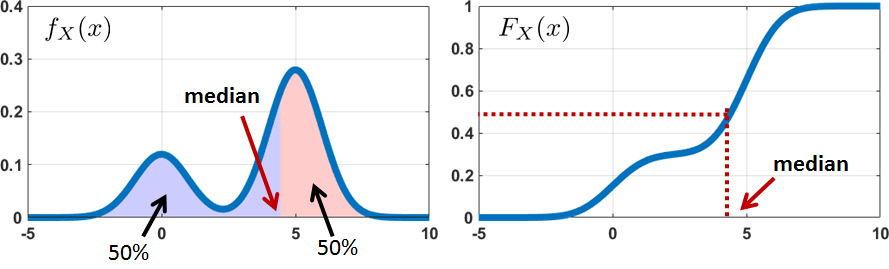
The median can also be evaluated from the CDF as follows.
The median of a random variable \(X\) is the point \(c\) such that
Proof. Since \(F_X(x) = \int_{-\infty}^{x} f_X(x') \;dx'\), we have
Rearranging the terms shows that \(F_X(c) = \frac{1}{2}\).
■- sep0ex
- Find a point \(c\) such that \(F_X(c) = 0.5\).
(Uniform random variable) Let \(X\) be a continuous random variable with PDF \(f_X(x) = \frac{1}{b-a}\) for \(a \le x \le b\), and is 0 otherwise. We know that the CDF of \(X\) is \(F_X(x) = \frac{x-a}{b-a}\) for \(a \le x \le b\). Therefore, the median of \(X\) is the number \(c \in \R\) such that \(F_X(c) = \frac{1}{2}\). Substituting into the CDF yields \(\frac{c-a}{b-a} = \frac{1}{2}\), which gives \(c = \frac{a+b}{2}\).
(Exponential random variable) Let \(X\) be a continuous random variable with PDF \(f_X(x) = \lambda e^{-\lambda x}\) for \(x \ge 0\). We know that the CDF of \(X\) is \(F_X(x) = 1-e^{-\lambda x}\) for \(x \ge 0\). The median of \(X\) is the point \(c\) such that \(F_X(c) = \frac{1}{2}\). This gives \(1-e^{-\lambda c} = \frac{1}{2}\), which is \(c = \frac{\log 2}{\lambda}\).
4.4.2Mode
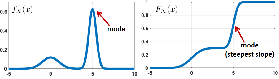
The mode is the peak of the PDF. We can see this from the definition below.
Let \(X\) be a continuous random variable. The mode is the point \(c\) such that \(f_X(x)\) attains the maximum:
The second equality holds because \(f_X(x) = F_X'(x) = \frac{d}{dx}\int_{-\infty}^x f_X(t)\;dt\). A pictorial illustration of mode is given in Figure 4.15. Note that the mode of a random variable is not unique, e.g., a mixture of two identical Gaussians with different means has two modes.
- sep0ex
- Find a point \(c\) such that \(f_X(c)\) is maximized.
How to find mode from CDF
- sep0ex
- Continuous: Find a point \(c\) such that \(F_X(c)\) has the steepest slope.
- Discrete: Find a point \(c\) such that \(F_X(c)\) has the biggest gap in a jump.
Let \(X\) be a continuous random variable with PDF \(f_X(x) = 6x(1-x)\) for \(0 \le x \le 1\). The mode of \(X\) happens at \(\argmax{x} \; f_X(x)\). To find this maximum, we take the derivative of \(f_X\). This gives
Setting this equal to zero yields \(x = \frac12\).
To ensure that this point is a maximum, we take the second-order derivative:
Therefore, we conclude that \(x = \frac12\) is a maximum point. Hence, the mode of \(X\) is \(x = \frac12\).
4.4.3Mean
We have defined the mean as the expectation of \(X\). Here, we show how to compute the expectation from the CDF. To simplify the demonstration, let us first assume that \(X > 0\).
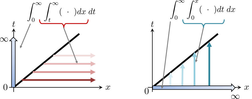
Let \(X> 0\). Then \(\E[X]\) can be computed from \(F_X\) as
Proof. The trick is to change the integration order:
Here, step \((a)\) is due to the change of integration order. See Figure 4.16 for an illustration.
■
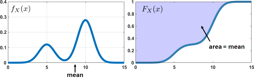
We draw a picture to illustrate the above lemma. As shown in Figure 4.17, the mean of a positive random variable \(X>0\) is equivalent to the area above the CDF.
Let \(X < 0\). Then \(\E[X]\) can be computed from \(F_X\) as
Proof. The idea here is also to change the integration order.
The mean of a random variable \(X\) can be computed from the CDF as
Proof. For any random variable \(X\), we can partition \(X = X^+ - X^-\) where \(X^+\) and \(X^-\) are the positive and negative parts, respectively. Then, the above two lemmas will give us
As illustrated in Figure 4.18, this equation is equivalent to computing the areas above and below the CDF and taking the difference.
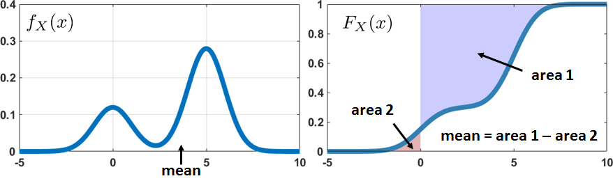
How to find the mean from the CDF
- sep0ex
A formula is given by Eq. (4.20):
$$\E[X] = \int_{0}^{\infty} \left(1-F_X(t)\right) \;dt - \int_{-\infty}^{0} F_X(t)\;dt.$$- This result is not commonly used, but the proof technique of switching the integration order is important.