Functions of Random Variables

One common question we encounter in practice is the transformation of random variables. The question can be summarized as follows: Given a random variable \(X\) with PDF \(f_X(x)\) and CDF \(F_X(x)\), and supposing that \(Y = g(X)\) for some function \(g\), what are \(f_Y(y)\) and \(F_Y(y)\)? This is a prevalent question. For example, we measure the voltage \(V\), and we want to analyze the power \(P = V^2/R\). This involves taking the square of a random variable. Another example: We know the distribution of the phase \(\Theta\), but we want to analyze the signal \(\cos(\omega t + \Theta)\). This involves a cosine transformation. How do we convert one variable to another? Answering this question is the goal of this section.

4.7.1General principle

We will first outline the general principle for tackling this type of problem. In the following subsection, we will give a few concrete examples.

Suppose we are given a random variable \(X\) with PDF \(f_X(x)\) and CDF \(F_X(x)\). Let \(Y = g(X)\) for some known and fixed function \(g\). For simplicity, we assume that \(g\) is monotonically increasing. In this case, the CDF of \(Y\) can be determined as follows.

This sequence of steps is not difficult to understand. Step (a) is the definition of CDF. Step (b) substitutes \(g(X)\) for \(Y\). Step (c) uses the fact that since \(g\) is invertible, we can apply the inverse of \(g\) to both sides of \(g(X)\le y\) to yield \(X \le g^{-1}(y)\). Step (d) is the definition of the CDF, but this time applied to \(\Pb[X \le \clubsuit] = F_X(\clubsuit)\), for some \(\clubsuit\).

It will be useful to visualize the situation in Figure 4.34. Here, we consider a uniformly distributed \(X\) so that the CDF \(F_X(x)\) is a straight line. According to \(F_X\), any samples drawn according to \(F_X\) are equally likely, as illustrated by the yellow dots on the \(x\)-axis. As we transform the \(X\)'s through \(Y = g(X)\), we increase/decrease the spacing between two samples. Therefore, some samples become more concentrated while some become less concentrated. The distribution of these transformed samples (the yellow dots on the \(y\)-axis) forms a new CDF \(F_Y(y)\). The result \(F_Y(y) = F_X(g^{-1}(y))\) holds when we look at \(Y\). The samples are traveling with \(g^{-1}\) in order to go back to \(F_X\). Therefore, we need \(g^{-1}\) in the formula.

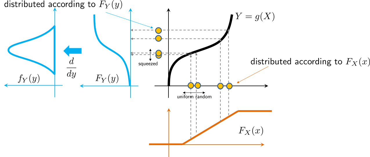
Why should we use the CDF and not the PDF in Figure 4.34? The advantage of the CDF is that it is an increasing function. Therefore, no matter what the function \(g\) is, the input and the output functions will still be increasing. If we use the PDF, then the non-monotonic behavior of the PDF will interact with another nonlinear function \(g\). It becomes much harder to decouple the two.

We can carry out the integrations to determine \(F_X(g^{-1}(y))\). It can be shown that

and hence, by the fundamental theorem of calculus, we have

where the last step is due to the chain rule. Based on this line of reasoning we can summarize a “recipe” for this problem.

This recipe works when \(g\) is a one-to-one mapping. If \(g\) is not one-to-one, e.g., \(g(x) = x^2\) implies \(g^{-1}(y) = \pm \sqrt{y}\), then we will have some issues with the above two steps. When this happens, then instead of writing \(X \le g^{-1}(y)\) we need to determine the set \(\{x \;|\; g(x) \le y\}\).

4.7.2Examples

Follow-Up. (Linear transformation of a Gaussian random variable). Suppose \(X\) is a Gaussian random variable with zero mean and unit variance, and let \(Y = aX + b\). Then the CDF and PDF of \(Y\) are respectively

Follow-Up. (Linear transformation of an exponential random variable). Suppose \(X\) is an exponential random variable with parameter \(\lambda\), and let \(Y = aX + b\). Then the CDF and PDF of \(Y\) are respectively

Example 4.27

Let \(X\) be a random variable with PDF \(f_X(x)\) and CDF \(F_X(x)\). Supposing that \(Y = X^2\), find \(f_Y(y)\) and \(F_Y(y)\). Express the answers in terms of \(f_X(x)\) and \(F_X(x)\).

Solution

We note that

$$\begin{aligned} F_Y(y) = \Pb[Y \le y] = \Pb[X^2 \le y] &= \Pb[-\sqrt{y} \le X \le \sqrt{y}] \\ &= F_X(\sqrt{y}) - F_X(-\sqrt{y}). \end{aligned}$$

Therefore, the PDF is

$$\begin{aligned} f_Y(y) &= \frac{d}{dy} F_Y(y) \\ &= \frac{d}{dy} \left(F_X(\sqrt{y}) - F_X(-\sqrt{y})\right) \\ &= F_X'(\sqrt{y}) \frac{d}{dy} \sqrt{y} - F_X'(-\sqrt{y}) \frac{d}{dy} \left(-\sqrt{y}\right)\\ &= \frac{1}{2\sqrt{y}}\left( f_X(\sqrt{y}) + f_X(-\sqrt{y})\right). \end{aligned}$$

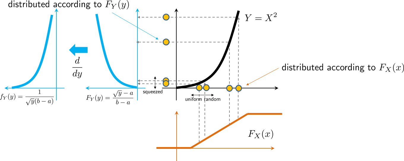
Follow Up. (Square of a uniform random variable) Suppose \(X\) is a uniform random variable in \([a,b]\) (assume \(a > 0\)), and let \(Y = X^2\). Then the CDF and PDF of \(Y\) are respectively

Closing remark. The transformation of random variables is a fundamental technique in data science. The approach we have presented is the most rudimentary yet the most intuitive. The key is to visualize the transformation and how the random samples are allocated after the transformation. Note that the density of the random samples is related to the slope of the CDF. Therefore, if the transformation maps many samples to similar values, the slope of the CDF will be steep. Once you understand this picture, the transformation will be a lot easier to understand.

Is it possible to replace the paper-and-pencil derivation of a transformation with a computer? If the objective is to transform random realizations, then the answer is yes because your goal is to transform numbers to numbers, which can be done on a computer. For example, transforming a sample \(x_1\) to \(\sqrt{x_1}\) is straightforward on a computer. However, if the objective is to derive the theoretical expression of the PDF, then the answer is no. Why might we want to derive the theoretical PDF? We might want to analyze the mean, variance, or other statistical properties. We may also want to reverse-engineer and determine a transformation that can yield a specific PDF. This would require a paper-and-pencil derivation. In what follows, we will discuss a handy application of the transformations.