eBook › Chapter 4 · Continuous Random Variables

Section 4.8

Generating Random Numbers

Most scientific computing software nowadays has built-in random number generators. For common types of random variables, e.g., Gaussian or exponential, these random number generators can easily generate numbers according to the chosen distribution. However, if we are given an arbitrary PDF (or PMF) that is not among the list of predefined distributions, how can we generate random numbers according to the PDF or PMF we want?

4.8.1General principle

Generating random numbers according to the desired distribution can be formulated as an inverse problem. Suppose that we can generate uniformly random numbers according to Uniform(0,1). This is a fair assumption, and this process can be done on almost all computers today. Let us call this random variable $U$ and its realization $u$. Suppose that we also have a desired distribution $f_X(x)$ (and its CDF $F_X(x)$). We can put the two random variables $U$ and $X$ on the two axes of Figure 4.36, yielding an input-output relationship. The inverse problem is: By using what transformation $g$, such that $X = g(U)$, can we make sure that $X$ is distributed according to $f_X(x)$ (or $F_X(x)$)?

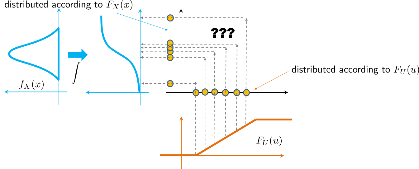
**Figure 4.36.** Generating random numbers according to a known CDF. The idea is to first generate a uniform(0,1) random variable, then do an inverse mapping $F_X^{-1}$.

Theorem 4.12

The transformation $g$ that can turn a uniform random variable into a random variable following a distribution $F_X(x)$ is given by

g(u) = F_X^{-1}(u).

That is, if $g = F_X^{-1}$, then $g(U)$ will be distributed according to $f_X$ (or $F_X$).

Proof. First, we know that if $U \sim \mathrm{Uniform}(0,1)$, then $f_U(u) = 1$ for $0 \le u \le 1$, so

\begin{aligned} F_U(u) = \int_{-\infty}^{u} f_U(u') \;du' = u, \end{aligned}

for $0 \le u \le 1$. Let $g = F^{-1}_X$ and define $Y = g(U)$. Then the CDF of $Y$ is

\begin{aligned} F_Y(y) = \Pb[Y \le y] &= \Pb[g(U) \le y] \\ &= \Pb[F_X^{-1}(U) \le y] \\ &= \Pb[U \le F_X(y)] = F_X(y). \end{aligned}

Therefore, we have shown that the CDF of $Y$ is the CDF of $X$.

■

The theorem above states that if we want a distribution $F_X$, then the transformation should be $g = F_X^{-1}$. This suggests a two-step process for generating random numbers.

How do we generate random numbers from an arbitrary distribution $F_X$?

sep0ex
Step 1: Generate a random number $U \sim \mathrm{Uniform}(0,1).$
Step 2: Let
$Y = F_X^{-1}(U).$
Then the distribution of $Y$ is $F_X$.

4.8.2Examples

Example 4.30

How can we generate Gaussian random numbers with mean $\mu$ and variance $\sigma^2$ from uniform random numbers?

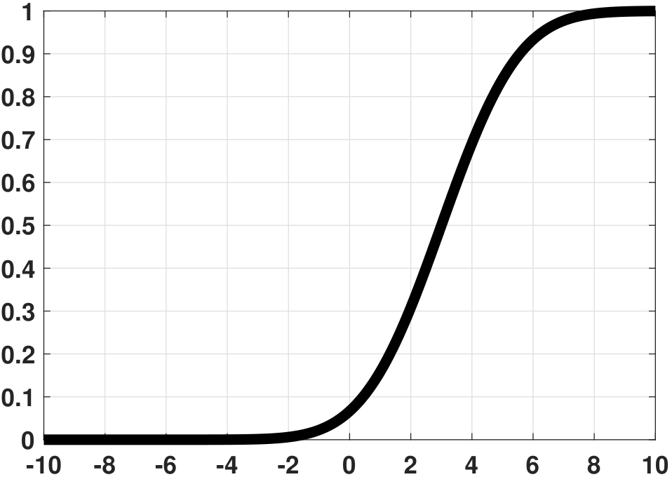
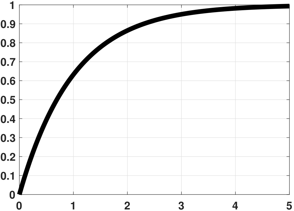
First, we generate $U \sim \text{Uniform}(0,1)$. The CDF of the ideal distribution is

F_X(x) = \Phi\left(\frac{x-\mu}{\sigma}\right).

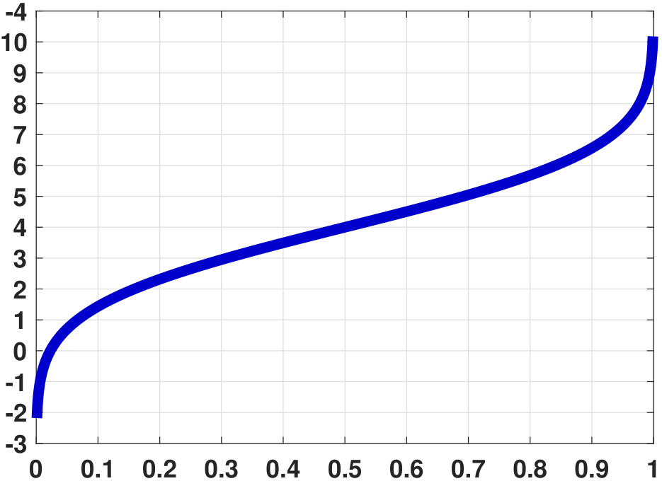
Therefore, the transformation $g$ is

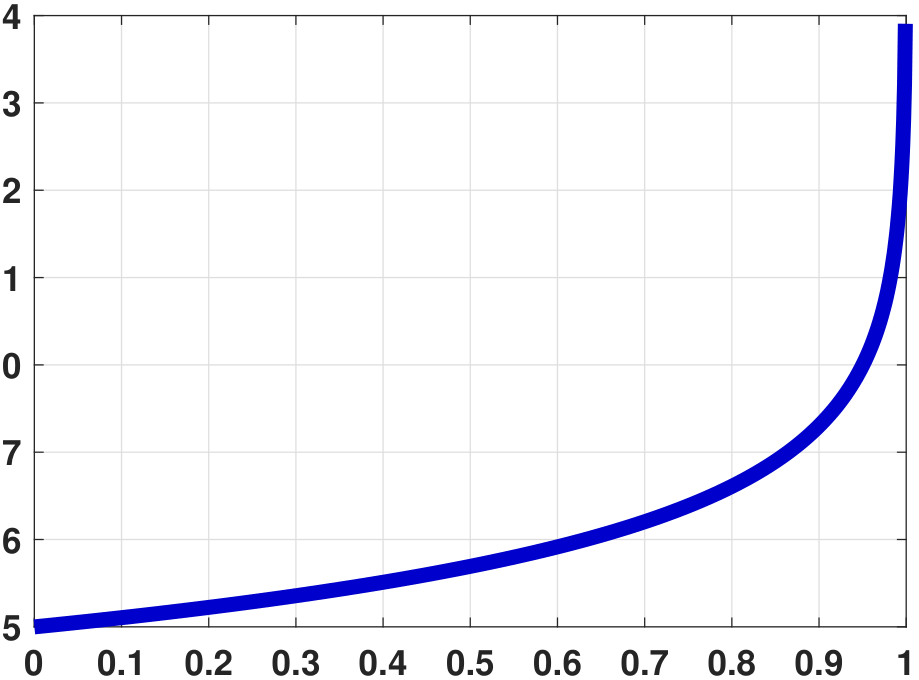
\begin{aligned} g(U) &= F_X^{-1}(U) = \sigma\Phi^{-1}(U) + \mu. \end{aligned}

In Figure 4.37, we plot the CDF of $F_X$ and the transformation $g$.

**Figure 4.37.** To generate random numbers according to a Gaussian, we plot its CDF in (a) and the transformation $g$ in (b).

To visualize the random variables before and after the transformation, we plot the histograms in Figure 4.38.

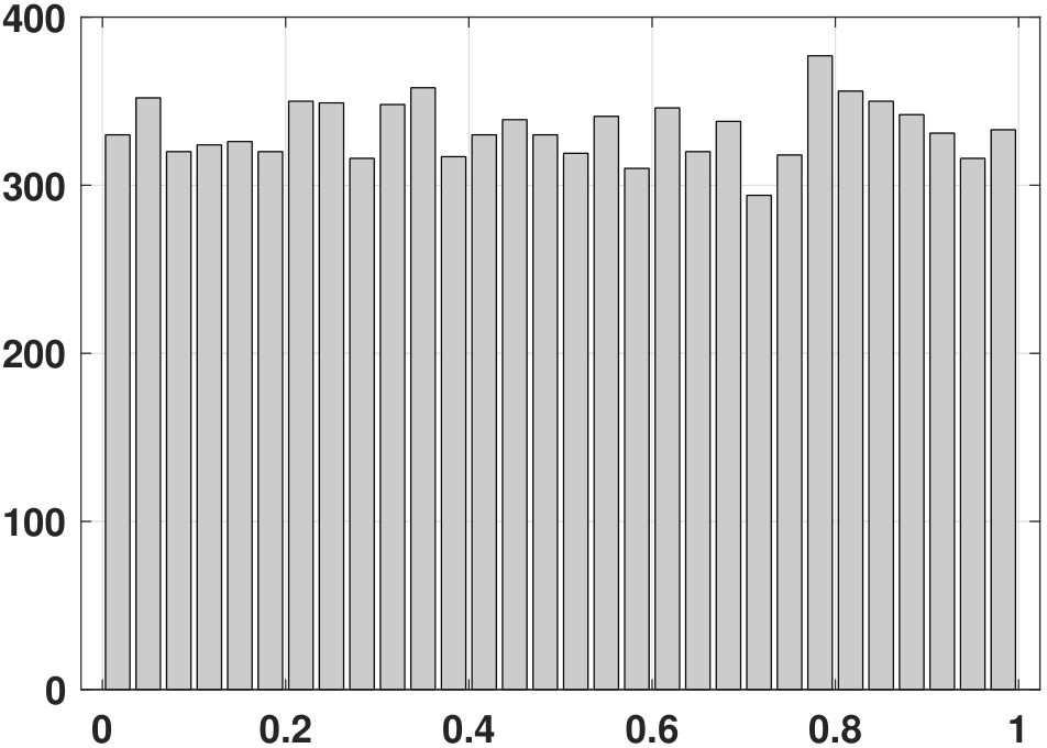
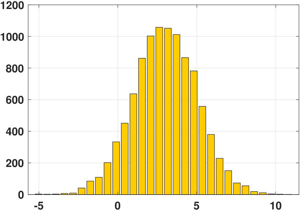
**Figure 4.38.** (a) PDF of the uniform random variable. (b) The PDF of the transformed random variable.

The MATLAB and Python codes used to generate the histograms above are shown below.

MATLAB

% MATLAB code to generate Gaussian from uniform
    mu    = 3;
    sigma = 2;
    U     = rand(10000,1);
    gU    = sigma*icdf('norm',U,0,1)+mu;
    figure; hist(U);
    figure; hist(gU);

Python

# Python code to generate Gaussian from uniform
    import numpy as np
    import matplotlib.pyplot as plt
    import scipy.stats as stats
    
    mu = 3
    sigma = 2
    U  = stats.uniform.rvs(0,1,size=10000)
    gU = sigma*stats.norm.ppf(U)+mu
    plt.hist(U); plt.show()
    plt.hist(gU); plt.show()

Example 4.31

How can we generate exponential random numbers with parameter $\lambda$ from uniform random numbers?

First, we generate $U \sim \text{Uniform}(0,1)$. The CDF of the ideal distribution is

F_X(x) = 1-e^{-\lambda x}.

Therefore, the transformation $g$ is

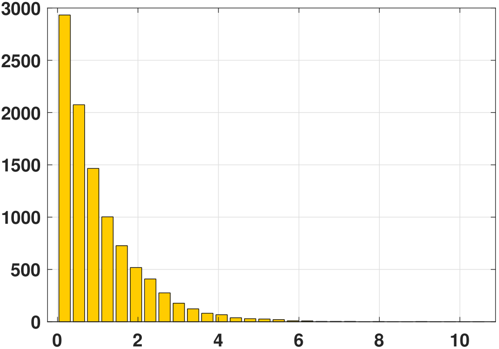
\begin{aligned} g(U) &= F_X^{-1}(U) = -\frac{1}{\lambda}\log(1-U). \end{aligned}

The CDF of the exponential random variable and the transformation $g$ are shown in Figure 4.39.

**Figure 4.39.** To generate random numbers according to $\text{Exponential}(1)$, we plot its CDF in (a) and the transformation $g$ in (b).

The PDF of the uniform random variable $U$ and the PDF of the transformed variable $g(U)$ are shown in Figure 4.40.

**Figure 4.40.** (a) PDF of the uniform random variable. (b) The PDF of the transformed random variable.

The MATLAB and Python codes for this transformation are shown below.

MATLAB

% MATLAB code to generate exponential random variables
    lambda = 1;
    U      = rand(10000,1);
    gU     = -(1/lambda)*log(1-U);

Python

# Python code to generate exponential random variables
    import numpy as np
    import scipy.stats as stats
    
    lambd = 1;
    U     = stats.uniform.rvs(0,1,size=10000)
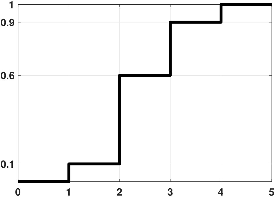
    gU    = -(1/lambd)*np.log(1-U)

Example 4.32

How can we generate the 4 integers $1,2,3,4$, according to the histogram $[0.1\; 0.5\; 0.3\; 0.1]$, from uniform random numbers?

First, we generate $U \sim \text{Uniform}(0,1)$. The CDF of the ideal distribution is

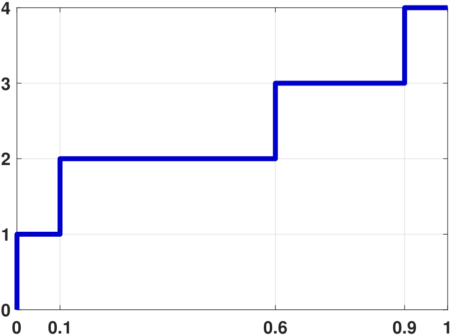
\begin{aligned} F_X(x) = \begin{cases} 0.1, &\qquad x = 1,\\ 0.1+0.5 = 0.6, &\qquad x = 2,\\ 0.1+0.5+0.3 = 0.9, &\qquad x = 3,\\ 0.1+0.5+0.3+0.1 = 1.0, &\qquad x = 4. \end{cases} \end{aligned}

This CDF is not invertible. However, we can still define the “inverse” mapping as

\begin{aligned} g(U) &= F_X^{-1}(U)\\ &= \begin{cases} 1, &\qquad 0.0 \le U \le 0.1,\\ 2, &\qquad 0.1 < U \le 0.6,\\ 3, &\qquad 0.6 < U \le 0.9,\\ 4, &\qquad 0.9 < U \le 1.0. \end{cases} \end{aligned}

For example, if $0.1 < U \le 0.6$, then on the black curve shown in Figure 4.41(a), we are looking at the second vertical line from the left. This will go to “2” on the $x$-axis. Therefore, the inversely mapped value is 2 for $0.1 < U \le 0.6$.

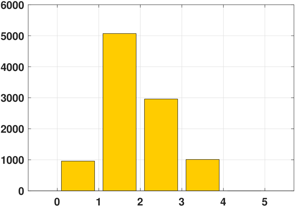
**Figure 4.41.** To generate random numbers according to a predefined histogram, we first define the CDF in (a) and the corresponding transformation in (b).

The PDFs of the transformed variables, before and after, are shown in Figure 4.42.

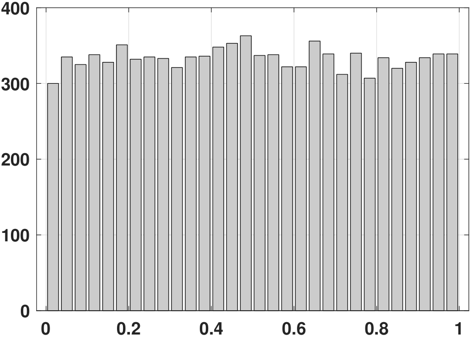
**Figure 4.42.** (a) PDF of the uniform random variable. (b) The PDF of the transformed random variable.

In MATLAB, the above PDFs can be plotted using the commands below. In Python, we need to use the logical comparison np.logical_and to identify the indices. An alternative is to use gU[((U<=0.5)*(U>=0.0)).astype(np.bool)]=1.

MATLAB

% MATLAB code to generate the desired random variables
    U  = rand(10000,1);
    gU = zeros(10000,1);
    gU((U>=0)  & (U<=0.1)) = 1;
    gU((U>0.1) & (U<=0.6)) = 2;
    gU((U>0.6) & (U<=0.9)) = 3;
    gU((U>0.9) & (U<=1))   = 4;

Python

# Python code to generate the desired random variables
    import numpy as np
    import scipy.stats as stats
    
    U  = stats.uniform.rvs(0,1,size=10000)
    gU = np.zeros(10000)
    gU[np.logical_and(U >= 0.0, U <= 0.1)] = 1
    gU[np.logical_and(U > 0.1, U <= 0.6)]  = 2
    gU[np.logical_and(U > 0.6, U <= 0.9)]  = 3
    gU[np.logical_and(U > 0.9, U <= 1)]    = 4