eBook › Chapter 5 · Joint Distributions

Section 5.2

Joint Expectation

5.2.1Definition and interpretation

When we have a single random variable, the expectation is defined as

\E[X] = \int_{\Omega} x f_X(x) \;dx.

For a pair of random variables, what would be a good way of defining the expectation? Certainly, we cannot just replace $f_X(x)$ by $f_{X,Y}(x,y)$ because the integration has to become a double integration. However, if it is a double integration, where should we put the variable $y$? It turns out that a useful way of defining the expectation for $X$ and $Y$ is as follows.

Definition 5.10

Let $X$ and $Y$ be two random variables. The joint expectation is

\E[XY] = \sum_{y \in \Omega_Y} \sum_{x \in \Omega_X} xy \;\cdot \; p_{X,Y}(x,y)

if $X$ and $Y$ are discrete, or

\E[XY] = \int_{y \in \Omega_Y} \int_{x \in \Omega_X} xy \;\cdot \; f_{X,Y}(x,y) \;dx\;dy

if $X$ and $Y$ are continuous. Joint expectation is also called correlation.

The double summation and integration on the right-hand side of the equation is nothing but the state times the probability. Here, the state is the product $xy$, and the probability is the joint PMF $p_{X,Y}(x,y)$ (or PDF). Therefore, as long as you agree that joint expectation should be defined as $\E[XY]$, the double summation and the double integration make sense.

The biggest mystery here is $\E[XY]$. You may wonder why the joint expectation should be defined as the expectation of the product $\E[XY]$. Why not the sum $\E[X+Y]$, or the difference $\E[X-Y]$, or the quotient $\E[X/Y]$? Why are we so deeply interested in $X$ times $Y$? These are excellent questions. That the joint expectation is defined as the product has to do with the correlation between two random variables. We will take a small detour into linear algebra.

Let us consider two discrete random variables $X$ and $Y$, both with $N$ states. So $X$ will take the states $\{x_1,x_2,\ldots,x_N\}$ and $Y$ will take the states $\{y_1,y_2,\ldots,y_N\}$. Let's define them as two vectors: $\vx \bydef [x_1,\ldots,x_N]^T$ and $\vy \bydef [y_1,\ldots,y_N]^T$. Since $X$ and $Y$ are random variables, they have a joint PMF $p_{X,Y}(x,y)$. The array of the PMF values can be written as a matrix:

\text{PMF as a matrix} = \mP \bydef \begin{bmatrix} p_{X,Y}(x_1,y_1) & p_{X,Y}(x_1,y_2) & \cdots & p_{X,Y}(x_1,y_N)\\ p_{X,Y}(x_2,y_1) & p_{X,Y}(x_2,y_2) & \cdots & p_{X,Y}(x_2,y_N)\\ \vdots & \vdots & \ddots & \vdots \\ p_{X,Y}(x_N,y_1) & p_{X,Y}(x_N,y_2) & \cdots & p_{X,Y}(x_N,y_N) \end{bmatrix}.

Let's try to write the joint expectation in terms of matrices and vectors. The definition of a joint expectation tells us that

\begin{aligned} \E[XY] &= \sum_{i = 1}^N \sum_{j = 1}^N x_i y_j \,\cdot \, p_{X,Y}(x_i,y_j), \end{aligned}

which can be written as

\begin{aligned} \E[XY] &= \underset{\vx^T}{\underbrace{\begin{bmatrix} x_1 & \cdots & x_N \end{bmatrix}}} \underset{\mP}{\underbrace{\begin{bmatrix} p_{X,Y}(x_1,y_1) & \cdots & p_{X,Y}(x_1,y_N)\\ \vdots & \ddots & \vdots \\ p_{X,Y}(x_N,y_1) & \cdots & p_{X,Y}(x_N,y_N) \end{bmatrix}}} \underset{\vy}{\underbrace{\begin{bmatrix} y_1\\ \vdots\\ y_N \end{bmatrix}}} = \vx^T\mP\vy. \end{aligned}

This is a weighted inner product between $\vx$ and $\vy$ using the weight matrix $\mP$.

Why correlation is defined as $\E[XY]$

sep0em
$\E[XY]$ is a weighted inner product between the states:
$\E[XY] = \vx^T\mP\vy.$
$\vx$ and $\vy$ are the states of the random variables $X$ and $Y$.
The inner product measures the similarity between two vectors.

Example 5.15

Let $X$ be a discrete random variable with $N$ states, where each state has an equal probability. Thus, $p_X(x) = 1/N$ for all $x$. Let $Y = X$ be another variable. Then the joint PMF of $(X,Y)$ is

p_{X,Y}(x,y) = \begin{cases} \frac{1}{N}, &\qquad x = y,\\ 0, &\qquad x\not= y. \end{cases}

It follows that the joint expectation is

\E[XY] = \sum_{i=1}^N \sum_{j=1}^N x_iy_j \cdot p_{X,Y}(x_i,y_j) = \frac{1}{N} \sum_{i=1}^N x_iy_i.

Equivalently, we can obtain the result via the inner product by defining

\mP = \begin{bmatrix} \frac{1}{N} & 0 & \cdots & 0\\ 0 & \frac{1}{N} & \cdots & 0\\ \vdots & \vdots & \ddots & \vdots \\ 0 & \cdots & \cdots & \frac{1}{N} \end{bmatrix} = \frac{1}{N}\mI.

In this case, the weighted inner product is $$\vx^T\mP\vy = \frac{\vx^T\vy}{N} = \frac{1}{N} \sum_{i=1}^N x_iy_i = \E[XY].$$

How do we understand the inner product? Ignoring the matrix $\mP$ for a moment, we recall an elementary result in linear algebra.

Definition 5.11

Let $\vx \in \R^N$ and $\vy \in \R^N$ be two vectors. Define the cosine angle $\cos\theta$ as

\cos\theta = \frac{\vx^T\vy}{\|\vx\|\|\vy\|},

where $\|\vx\| = \sqrt{\sum_{i=1}^Nx_i^2}$ is the norm of the vector $\vx$, and $\|\vy\| = \sqrt{\sum_{i=1}^N y_i^2}$ is the norm of the vector $\vy$.

This definition can be understood as the geometry between two vectors, as illustrated in Figure 5.7. If the two vectors $\vx$ and $\vy$ are parallel so that $\vx = \alpha\vy$ for some $\alpha$, then the angle $\theta = 0$. If $\vx$ and $\vy$ are orthogonal so that $\vx^T\vy = 0$, then $\theta = \pi/2$. Therefore, the inner product $\vx^T\vy$ tells us the degree of correlation between the vectors $\vx$ and $\vy$.

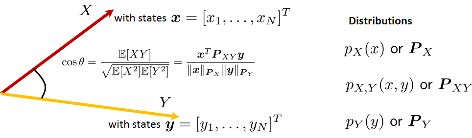
Now let's come back to our discussion about the joint expectation. The cosine angle definition tells us that if $\E[XY] = \vx^T\mP\vy$, the following form would make sense:

\cos\theta = \frac{\vx^T\mP\vy}{\|\vx\|\|\vy\|} = \frac{\E[XY]}{\|\vx\|\|\vy\|}.

That is, as long as we can find out the norms $\|\vx\|$ and $\|\vy\|$, we will be able to interpret $\E[XY]$ from the cosine angle perspective. But what would be a reasonable definition of $\|\vx\|$ and $\|\vy\|$? We define the norm by first considering the variance of the random variable $X$ and $Y$:

\begin{aligned} \E[X^2] &= \sum_{i = 1}^N x_i x_i \,\cdot \, p_{X}(x_i)\\ &= \underset{\vx^T}{\underbrace{\begin{bmatrix} x_1 & \cdots & x_N \end{bmatrix}}} \underset{\mP_X}{\underbrace{\begin{bmatrix} p_{X}(x_1) & \cdots & 0\\ \vdots & \ddots & \vdots \\ 0 & \cdots & p_{X}(x_N) \end{bmatrix}}} \underset{\vx}{\underbrace{\begin{bmatrix} x_1\\ \vdots\\ x_N \end{bmatrix}}} \\ &= \vx^T\mP_{X}\vx = \|\vx\|_{\mP_X}^2, \end{aligned}

where $\mP_X$ is the diagonal matrix storing the probability masses of the random variable $X$. It is not difficult to show that $\mP_X = \text{diag}(\mP\vone)$ by following the definition of the marginal distributions (which are the column and row sums of the joint PMF). Similarly we can define

\begin{aligned} \E[Y^2] &= \sum_{j = 1}^N y_j y_j \,\cdot \, p_{Y}(y_j)\\ &= \underset{\vy^T}{\underbrace{\begin{bmatrix} y_1 & \cdots & y_N \end{bmatrix}}} \underset{\mP_Y}{\underbrace{\begin{bmatrix} p_{Y}(y_1) & \cdots & 0\\ \vdots & \ddots & \vdots \\ 0 & \cdots & p_{Y}(y_N) \end{bmatrix}}} \underset{\vy}{\underbrace{\begin{bmatrix} y_1\\ \vdots\\ y_N \end{bmatrix}}} \\ &= \vy^T\mP_{Y}\vy = \|\vy\|_{\mP_Y}^2. \end{aligned}

Therefore, one way to define the cosine angle is to start with

\cos\theta = \frac{\vx^T\mP_{XY}\vy}{\|\vx\|_{\mP_X}\|\vy\|_{\mP_Y}},

where $\mP_{XY} = \mP$, $\|\vx\|_{\mP_X} = \sqrt{\vx^T\mP_X\vx}$ and $\|\vy\|_{\mP_Y} = \sqrt{\vy^T\mP_Y\vy}$. But writing it in terms of the expectation, we observe that this cosine angle is exactly

\begin{aligned} \cos\theta &= \frac{\vx^T\mP_{XY}\vy}{\|\vx\|_{\mP_X}\|\vy\|_{\mP_Y}} \\ &= \frac{\E[XY]}{\sqrt{\E[X^2]}\sqrt{\E[Y^2]}}. \end{aligned}

Therefore, $\E[XY]$ defines the cosine angle between the two random variables, which, in turn, defines the correlation between the two. A large $|\E[XY]|$ means that $X$ and $Y$ are highly correlated, and a small $|\E[XY]|$ means that $X$ and $Y$ are not very correlated. If $\E[XY] = 0$, then the two random variables are uncorrelated. Therefore, $\E[XY]$ tells us how the two random variables are related to each other.

To further convince you that $ [XY]{[X^2][Y^2]} $ can be interpreted as a cosine angle, we show that

-1 \le \frac{\E[XY]}{\sqrt{\E[X^2]}\sqrt{\E[Y^2]}} \le 1,

because if this ratio can go beyond $+1$ and $-1$, it makes no sense to call it a cosine angle. The argument follows from a very well-known inequality in probability, called the Cauchy-Schwarz inequality (for expectation), which states that $ -1 [XY]{[X^2][Y^2]} 1 $:

Theorem 5.2 (Cauchy-Schwarz inequality)

For any random variables $X$ and $Y$,

(\E[XY])^2 \le \E[X^2]\E[Y^2].

The following proof can be skipped if you are reading the book the first time.

Proof. Let $t\in \R$ be a constant. Consider

\begin{aligned} \E[(X+tY)^2] = \E[X^2 + 2tXY + t^2Y^2]. \end{aligned}

Since $\E[(X+tY)^2] \ge 0$ for any $t$, it follows that

\begin{aligned} \E[X^2 + 2tXY + t^2Y^2] \ge 0. \end{aligned}

Expanding the left-hand side yields

\begin{aligned} t^2\E[Y^2] + 2t \E[XY] + \E[X^2] \ge 0. \end{aligned}

This is a quadratic equation in $t$, and we know that for any quadratic equation $a t^2 + bt + c \ge 0$ we must have $b^2 - 4ac \le 0$. Therefore, in our case, we have that

(2\E[XY])^2 - 4\E[Y^2]\E[X^2] \le 0,

which means $(\E[XY])^2 \le \E[X^2]\E[Y^2]$. The equality holds when $\E[(X+tY)^2] = 0$. In this case, $X = -tY$ for some $t$, i.e., the random variable $X$ is a scaled version of $Y$ so that the vector formed by the states of $X$ is parallel to that of $Y$.

■

End of the proof.

5.2.2Covariance and correlation coefficient

In many practical problems, we prefer to work with central moments, i.e., $\E[(X - \mu_X)^2]$ instead of $\E[X^2]$. This essentially means that we subtract the mean from the random variable. If we adopt such a centralized random variable, we can define the covariance as follows.

Definition 5.12

Let $X$ and $Y$ be two random variables. Then the covariance of $X$ and $Y$ is

\Cov(X,Y) = \E[(X-\mu_X)(Y-\mu_Y)],

where $\mu_X = \E[X]$ and $\mu_Y = \E[Y]$.

It is easy to show that if $X = Y$, then the covariance simplifies to the variance:

\begin{aligned} \Cov(X,X) &= \E[(X-\mu_X)(X-\mu_X)] = \Var[X]. \end{aligned}

Thus, covariance is a generalization of variance. The former can handle a pair of variables, whereas the latter is only for a single variable. We can also demonstrate the following result.

Theorem 5.3

Let $X$ and $Y$ be two random variables. Then

\Cov(X,Y) = \E[XY] - \E[X]\E[Y].

Proof. Just apply the definition of covariance:

\begin{aligned} \Cov(X,Y) &= \E[(X-\mu_X)(Y-\mu_Y)] \\ &= \E[XY - X\mu_Y - Y \mu_X + \mu_X\mu_Y] = \E[XY] - \mu_X\mu_Y. \end{aligned}

■

The next theorem concerns the sum of two random variables.

Theorem 5.4

For any $X$ and $Y$,

[a.] $\E[X+Y]=\E[X]+\E[Y].$
[b.] $\Var[X+Y] = \Var[X] + 2\Cov(X,Y) + \Var[Y].$

Proof. Recall the definition of joint expectation:

\begin{aligned} \E[X+Y] &= \sum_{y}\sum_{x} (x+y)p_{X,Y}(x,y) \\ &= \sum_{y} \sum_{x} xp_{X,Y}(x,y) + \sum_{y} \sum_{x} y p_{X,Y}(x,y)\\ &= \sum_{x} x \left(\sum_{y} p_{X,Y}(x,y)\right) + \sum_{y} y \left(\sum_{x} p_{X,Y}(x,y)\right)\\ &= \sum_x x p_X(x) + \sum_y yp_Y(y) \\ &= \E[X] + \E[Y]. \end{aligned}

Similarly,

\begin{aligned} \Var[X+Y] &= \E[(X+Y)^2] - \E[X+Y]^2 \\ &= \E[(X+Y)^2] - (\mu_X+\mu_Y)^2 \\ &= \E[X^2 + 2XY + Y^2] - (\mu_X^2+ 2\mu_X\mu_Y + \mu_Y^2) \\ &= \E[X^2]-\mu_X^2 + \E[Y^2] - \mu_Y^2 + 2(\E[XY]-\mu_X\mu_Y)\\ &= \Var[X] + 2\Cov(X,Y) + \Var[Y]. \end{aligned}

■

With covariance defined, we can now define the correlation coefficient $\rho$, which is the cosine angle of the centralized variables. That is,

\begin{aligned} \rho &= \cos\theta \\ &= \frac{\E[(X-\mu_X)(Y-\mu_Y)]}{\sqrt{\E[(X-\mu_X)^2]\E[(Y-\mu_Y)^2]}}. \end{aligned}

Recognizing that the denominator of this expression is just the variance of $X$ and $Y$, we define the correlation coefficient as follows.

Definition 5.13

Let $X$ and $Y$ be two random variables. The correlation coefficient is

\rho = \frac{\Cov(X,Y)}{\sqrt{\Var[X]\Var[Y]}}.

Since $-1\le \cos\theta \le 1$, $\rho$ is also between $-1$ and $1$. The difference between $\rho$ and $\E[XY]$ is that $\rho$ is normalized with respect to the variance of $X$ and $Y$, whereas $\E[XY]$ is not normalized. The correlation coefficient has the following properties:

sep0ex
$\rho$ is always between $-1$ and $1$, i.e., $-1 \le \rho \le 1$. This is due to the cosine angle definition.
When $X = Y$ (fully correlated), $\rho = +1$.
When $X = -Y$ (negatively correlated), $\rho = -1$.
When $X$ and $Y$ are uncorrelated, $\rho = 0$.

5.2.3Independence and correlation

If two random variables $X$ and $Y$ are independent, the joint expectation can be written as a product of two individual expectations.

Theorem 5.5

If $X$ and $Y$ are independent, then

\E[XY] = \E[X]\E[Y].

Proof. We only prove the discrete case because the continuous can be proved similarly. If $X$ and $Y$ are independent, we have $p_{X,Y}(x,y) = p_X(x)\;p_Y(y)$. Therefore,

\begin{aligned} \E[XY] = \sum_{y}\sum_{x} xy p_{X,Y}(x,y) &= \sum_{y} \sum_x xy p_{X}(x)p_Y(y) \\ &= \left(\sum_x x p_{X}(x)\right) \left(\sum_y y p_{Y}(y)\right) = \E[X]\E[Y]. \end{aligned}

■

In general, for any two independent random variables and two functions $f$ and $g$,

\E[f(X)g(Y)] = \E[f(X)]\E[g(Y)].

The following theorem illustrates a few important relationships between independence and correlation.

Theorem 5.6

Consider the following two statements:

[a.] $X$ and $Y$ are independent;
[b.] $\Cov(X,Y) = 0$.

Statement (a) implies statement (b), but (b) does not imply (a). Thus, independence is a stronger condition than correlation.

Proof. We first prove that (a) implies (b). If $X$ and $Y$ are independent, then $\E[XY] = \E[X]\E[Y]$. In this case,

\begin{aligned} \Cov(X,Y) = \E[XY]-\E[X]\E[Y] = \E[X]\E[Y] - \E[X]\E[Y] = 0. \end{aligned}

To prove that (b) does not imply (a), we show a counterexample. Consider a discrete random variable $Z$ with PMF

p_Z(z) = \begin{bmatrix} \frac{1}{4} & \frac{1}{4} & \frac{1}{4} & \frac{1}{4} \end{bmatrix}.

Let $X$ and $Y$ be

X = \cos \frac{\pi}{2}Z \quad\mbox{and}\quad Y = \sin \frac{\pi}{2}Z.

Then we can show that $\E[X] = 0$ and $\E[Y] = 0$. The covariance is

\begin{aligned} \Cov(X,Y) &= \E[(X-0)(Y-0)] \\ &= \E\left[ \cos \frac{\pi}{2}Z \sin \frac{\pi}{2}Z\right] \\ &= \E\left[\frac{1}{2}\sin \pi Z\right] \\ &= \frac{1}{2}\left[ (\sin \pi 0) \frac{1}{4} + (\sin \pi 1) \frac{1}{4} + (\sin \pi 2) \frac{1}{4} + (\sin \pi 3) \frac{1}{4}\right] = 0. \end{aligned}

The next step is to show that $X$ and $Y$ are dependent. To this end, we only need to show that $p_{X,Y}(x,y) \not= p_X(x)p_Y(y)$. The joint PMF $p_{X,Y}(x,y)$ can be found by noting that

\begin{aligned} Z = 0 &\Rightarrow X = 1,\ Y = 0, \\ Z = 1 &\Rightarrow X = 0,\ Y = 1, \\ Z = 2 &\Rightarrow X = -1,\ Y = 0, \\ Z = 3 &\Rightarrow X = 0,\ Y = -1. \end{aligned}

Thus, the PMF is

p_{X,Y}(x,y) = \begin{bmatrix} 0 & \frac{1}{4} & 0 \\ \frac{1}{4} & 0 & \frac{1}{4}\\ 0 & \frac{1}{4} & 0 \end{bmatrix}.

The marginal PMFs are

\begin{aligned} p_X(x) = \begin{bmatrix} \frac{1}{4} & \frac{1}{2} & \frac{1}{4} \end{bmatrix}, \quad p_Y(y) = \begin{bmatrix} \frac{1}{4} & \frac{1}{2} & \frac{1}{4} \end{bmatrix}. \end{aligned}

The product $p_X(x)\;p_Y(y)$ is

p_X(x)p_Y(y) = \begin{bmatrix} \frac{1}{16} & \tfrac{1}{8} & \tfrac{1}{16} \\[0.5em] \frac{1}{8} & \tfrac{1}{4} & \tfrac{1}{8}\\[0.5em] \frac{1}{16} & \tfrac{1}{8} & \tfrac{1}{16} \end{bmatrix}.

Therefore, $p_{X,Y}(x,y) \not= p_X(x)p_Y(y)$, although $\E[XY] = \E[X]\E[Y]$.

■

What is the relationship between independent and uncorrelated?

sep0em
Independent $\Rightarrow$ uncorrelated.
Independent $\nLeftarrow$ uncorrelated.

5.2.4Computing correlation from data

We close this section by discussing a very practical problem: Given a dataset containing two columns of data points, how do we determine whether the two columns are correlated?

Recall that the correlation coefficient is defined as

\rho = \frac{\E[XY]-\mu_X\mu_Y}{\sigma_X\sigma_Y}.

If we have a dataset containing $(x_n,y_n)_{n=1}^N$, then the correlation coefficient can be approximated by

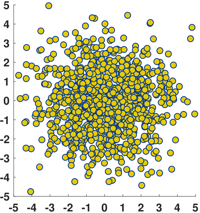
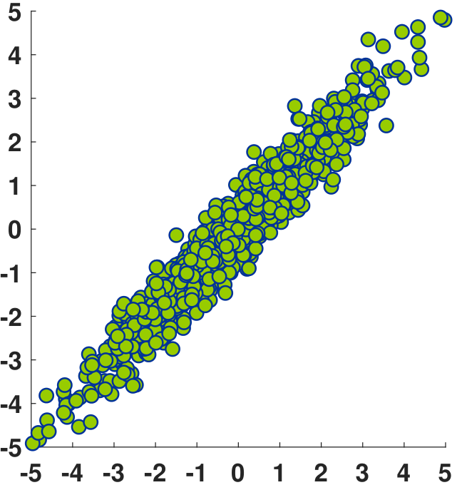
\widehat{\rho} = \frac{\frac{1}{N}\sum_{n=1}^N x_ny_n - \overline{x} \,\overline{y}}{ \sqrt{\frac{1}{N}\sum_{n=1}^N(x_n-\overline{x})^2} \sqrt{\frac{1}{N}\sum_{n=1}^N(y_n-\overline{y})^2}},

where $\overline{x} = \frac{1}{N}\sum_{n=1}^N x_n$ and $\overline{y} = \frac{1}{N}\sum_{n=1}^N y_n$ are the means. This equation should not be a surprise because essentially all terms are the empirical estimates. Thus, $\widehat{\rho}$ is the empirical correlation coefficient determined from the dataset. As $N \rightarrow \infty$, we expect $\widehat{\rho} \rightarrow \rho$. Figure 5.8 shows three example datasets. We plot the $(x_n,y_n)$ pairs as coordinates in the 2D plane. The first dataset contains samples that are almost uncorrelated. We can see that $x_n$ does not tell us anything about $y_n$. The second dataset is moderately correlated. The third dataset is highly correlated: If we know $x_n$, we are almost certain to know the corresponding $y_n$, with a small number of perturbations.

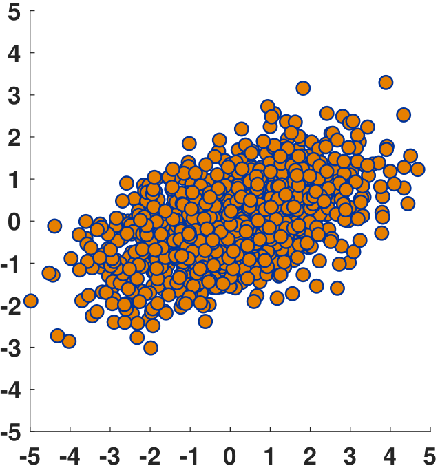
**Figure 5.8.** Visualization of correlated variables. Each of these figures represent a scattered plot of a dataset containing $(x_n,y_n)_{n=1}^N$. (a) is uncorrelated. (b) is somewhat correlated. (c) is strongly correlated.

On a computer, computing the correlation coefficient can be done using built-in commands such as corrcoef in MATLAB and stats.pearsonr in Python. The codes to generate the results in Figure 5.8(b) are shown below.

MATLAB

% MATLAB code to compute the correlation coefficient
    x = mvnrnd([0,0],[3 1; 1 1],1000);
    figure(1); scatter(x(:,1),x(:,2));
    rho = corrcoef(x)

Python

# Python code to compute the correlation coefficient
    import numpy as np
    import scipy.stats as stats
    import matplotlib.pyplot as plt
    x = stats.multivariate_normal.rvs([0,0], [[3,1],[1,1]], 10000)
    plt.figure(); plt.scatter(x[:,0],x[:,1])
    rho,_ = stats.pearsonr(x[:,0],x[:,1])
    print(rho)