eBook › Chapter 5 · Joint Distributions

Section 5.6

Random Vectors and Covariance Matrices

We now enter the second part of this chapter. In the first part, we were mainly interested in a pair of random variables. In the second part, however, we will study vectors of \(N\) random variables. To understand a vector of random variables, we will not drill down to the integrations of the PDFs (which you would certainly not enjoy). Instead, we will blend linear algebra tools and probabilistic tools to learn a few practical data analysis techniques.

5.6.1PDF of random vectors

Joint distributions can be generalized to more than two random variables. The most convenient way is to consider a vector of random variables and their corresponding states.

\mX = \begin{bmatrix}X_1 \\ X_2 \\ \vdots \\ X_N \end{bmatrix} \quad\mbox{and}\quad \vx = \begin{bmatrix}x_1 \\ x_2 \\ \vdots \\ x_N \end{bmatrix}.

Our notation here is unconventional since bold upper case letters usually represent matrices. Here, \(\mX\) denotes a vector, specifically a random vector. Its state is a vector \(\vx\). In this chapter, we will use the following notational convention: \(\mX\) and \(\mY\) represent random vectors while \(\mA\) represents a matrix.

One way to think about \(\mX\) is to imagine that if you put your hand into the sample space, you will pick up a vector \(\vx\). This random realization \(\vx\) has \(N\) entries, and so you need to specify the probability of getting all of these entries simultaneously. Accordingly, we should expect that \(\mX\) is characterized by an \(N\)-dimensional PDF

f_{\mX}(\vx) = f_{X_1,X_2,\ldots,X_N}(x_1,x_2,\ldots,x_N).

Essentially, this PDF tells us the probability density for random variable \(X_1 = x_1\), random variable \(X_2 = x_2\), etc. It is a coordinate-wise description. For example, if \(\mX\) contains three elements such that \(\mX = [X_1,X_2,X_3]^T\), and if the state we are looking at is \(\vx = [3, \, 1,\, 7]^T\), then \(f_{\mX}(\vx)\) is the probability density such that this 3D coordinate \((X_1,X_2,X_3)\) takes the value \([3,1,7]^T\).

To compute the probability, we can integrate \(f_{\mX}(\vx)\) with respect to \(\vx\). Let \(\calA\) be the event. Then

\begin{aligned} \Pb[\mX \in \calA] &= \int_\calA f_{\mX}(\vx)\;d\vx \\ &= \int \cdots \int_\calA f_{X_1,\ldots,X_N}(x_1,\ldots,x_N)\;dx_1\ldots d x_N. \end{aligned}

If the random coordinates \(X_1,\ldots,X_N\) are independent, the PDF can be written as a product of \(N\) individual PDFs:

\begin{aligned} f_{X_1,\ldots,X_N}(x_1,\ldots,x_N) &= f_{X_1}(x_1) f_{X_2}(x_2) \cdots f_{X_N}(x_N), \; \text{and so} \; \\ \Pb[\mX \in \calA] &= \int \cdots \int_\calA f_{X_1}(x_1) f_{X_2}(x_2) \cdots f_{X_N}(x_N) \;dx_1 \cdots d x_N. \end{aligned}

However, this does not necessarily simplify the calculation unless \(\calA\) is separable, e.g., \(\calA = [a_1,b_1]\times[a_2,b_2]\times\cdots\times[a_N,b_N]\). In this case, the integration becomes

\begin{aligned} \Pb[\mX \in \calA] &= \prod_{i=1}^N \left[\int_{a_i}^{b_i} f_{X_i}(x_i) \;dx_i\right], \end{aligned}

which is obviously manageable.

Example 5.24

Let \(\mX = [X_1,\ldots,X_N]^T\) be a vector of zero-mean unit-variance Gaussian random variables. Let \(\calA = [-1,2]^N\). Then

\begin{aligned} \Pb[\mX \in \calA] &= \int_\calA f_{\mX}(\vx)d\vx \\ &= \int \cdots \int_\calA f_{X_1,\cdots,X_N}(x_1,\ldots,x_N)\;dx_1\cdots d x_N\\ &= \left[\int_{-1}^{2} f_{X_1}(x_1)\;dx_1\right]^N = \left[\Phi(2)-\Phi(-1)\right]^N, \end{aligned}

where \(\Phi(\cdot)\) is the standard Gaussian CDF.

As you can see from the definition of a vector random variable, computing the probability typically involves integrating a high-dimensional function, which is tedious. However, the good news is that in practice we seldom need to perform such calculations. Often we are more interested in the mean and the covariance of the random vectors because they usually carry geometric meanings. The next subsection explores this topic.

5.6.2Expectation of random vectors

Let \(\mX = [X_1,\ldots,X_N]^T\) be a random vector. We define the expectation of a random vector as follows.

Definition 5.19

Let \(\mX = [X_1,\ldots,X_N]^T\) be a random vector. The expectation is

\vmu \bydef \E[\mX] = \begin{bmatrix}\E[X_1]\\ \E[X_2] \\ \vdots \\ \E[X_N]\end{bmatrix}.

The resulting vector is called the mean vector. Since the mean vector is a vector of individual elements, we need to compute the marginal PDFs before computing the expectations:

\E[\mX] = \begin{bmatrix} \E[X_1]\\ \vdots\\ \E[X_N] \end{bmatrix} = \begin{bmatrix} \int_{\Omega} x_1 f_{X_1}(x_1) \;dx_1\\ \vdots\\ \int_{\Omega} x_N f_{X_N}(x_N) \;dx_N \end{bmatrix},

where the marginal PDF is determined by

f_{X_n}(x_n) = \int_{\Omega} f_{\mX}(\vx) \,d\vx_{\backslash n}.

In the equation above, \(\vx_{\backslash n} = [x_1,\ldots,x_{n-1},x_{n+1},\ldots,x_N]^T\) contains all the elements without \(x_n\). For example, if the PDF is \(f_{X_1,X_2,X_3}(x_1,x_2,x_3)\), then

\begin{aligned} \E[X_1] &= \int x_1 \;\; \underset{\textcolor{myblue}{f_{X_1}(x_1)}}{\underbrace{\int f_{X_1,X_2,X_3}(x_1,x_2,x_3) \;dx_2\;dx_3}} \;\; \;dx_1. \end{aligned}

Again, this will become tedious when there are many variables.

While the definition of the expectation may be challenging to understand, some problems using it are straightforward. We will first demonstrate the case of independent Poisson random variables, and then we will discuss joint Gaussians.

Example 5.25

Let \(\mX = [X_1,\ldots,X_N]^T\) be a random vector such that \(X_n\) are independent Poissons with \(X_n \sim \text{Poisson}(\lambda_n)\). Then

\begin{aligned} \E[\mX] &= \begin{bmatrix} \E[X_1]\\ \vdots\\ \E[X_N] \end{bmatrix} = \begin{bmatrix} \sum_{k=0}^{\infty} k \cdot \frac{\lambda_1^k e^{-\lambda_1}}{k!}\\ \vdots\\ \sum_{k=0}^{\infty} k \cdot \frac{\lambda_N^k e^{-\lambda_N}}{k!} \end{bmatrix} = \begin{bmatrix} \lambda_1\\ \vdots \\ \lambda_N \end{bmatrix}. \end{aligned}

On computers, computing the mean vector can be done using built-in commands such as mean in MATLAB and np.mean in Python. However, caution is needed when performing the calculation. In MATLAB, mean computes along first dimension (rows index). Thus, if we have an \(N \times 2\) array, applying mean will give us a \(1 \times 2\) vector. To obtain the column mean vector of size \(N \times 1\), we need to specify the direction as mean(X,2). Similarly, in Python, when calling np.mean, we need to specify the axis.

MATLAB

% MATLAB code to compute a mean vector
    X    = randn(100,2);
    mX   = mean(X,2);

Python

# Python code to compute a mean vector
    import numpy as np
    import scipy.stats as stats
    X = stats.multivariate_normal.rvs([0,0],[[1,0],[0,1]],100)
    mX = np.mean(X,axis=1)

5.6.3Covariance matrix

Definition 5.20

The covariance matrix of a random vector \(\mX = [X_1,\ldots,X_N]^T\) is

\mSigma \bydef \Cov(\mX) = \begin{bmatrix} \Var[X_1] & \Cov(X_1,X_2) & \cdots & \Cov(X_1,X_N) \\ \Cov(X_2,X_1) & \Var[X_2] & \cdots & \Cov(X_2,X_N) \\ \vdots & \vdots & \ddots & \vdots \\ \Cov(X_N,X_1) & \Cov(X_N,X_2) & \cdots & \Var[X_N] \end{bmatrix}.

A more compact way of writing the covariance matrix is

\mSigma = \Cov(\mX) = \E[(\mX-\vmu)(\mX-\vmu)^T],

where \(\vmu = \E[\mX]\) is the mean vector. The notation \(\va\vb^T\) means the outer product, defined as

\begin{aligned} \va\vb^T = \begin{bmatrix} a_1\\ \vdots\\ a_N \end{bmatrix} \begin{bmatrix} b_1 & \cdots & b_N \end{bmatrix} = \begin{bmatrix} a_1b_1 & a_1b_2 & \cdots & a_1b_N\\ \vdots & \vdots & \ddots & \vdots \\ a_Nb_1 & a_Nb_2 & \cdots & a_Nb_N \end{bmatrix}. \end{aligned}

It is easy to show that \(\Cov(\mX) = \Cov(\mX)^T\), i.e., they are symmetric.

Theorem 5.13

If the coordinates \(X_1,\ldots,X_N\) are independent, then the covariance matrix \(\Cov(\mX) = \mSigma\) is a diagonal matrix:

\begin{aligned} \mSigma = \Cov(\mX) = \begin{bmatrix} \Var[X_1] & 0 & \cdots & 0 \\ 0 & \Var[X_2] & \cdots & 0 \\ \vdots & \vdots & \ddots & \vdots \\ 0 & 0 & \cdots & \Var[X_N] \end{bmatrix}. \end{aligned}

Proof. If all \(X_i\)'s are independent, then \(\Cov(X_i,X_j) = 0\) for all \(i \not= j\). Substituting this into the definition of the covariance matrix, we obtain the result.

■

If we ignore the mean vector \(\vmu\), we obtain the autocorrelation matrix \(\mR\).

Definition 5.21

Let \(\mX = [X_1,\ldots,X_N]^T\) be a random vector. The autocorrelation matrix is

\mR = \E[\mX\mX^T] = \begin{bmatrix} \E[X_1X_1] & \E[X_1X_2] & \cdots & \E[X_1X_N] \\ \E[X_2X_1] & \E[X_2X_2] & \cdots & \E[X_2X_N] \\ \vdots & \vdots & \ddots & \vdots \\ \E[X_NX_1] & \E[X_NX_2] & \cdots & \E[X_NX_N] \end{bmatrix}.

We state without proof that

\mSigma = \mR - \vmu\vmu^T,

which corresponds to the single-variable case where \(\sigma^2 = \E[X^2]-\mu^2\).

On computers, computing the covariance matrix is done using built-in commands cov in MATLAB and np.cov in Python. Like the mean vectors, when computing the covariance, we need to specify the direction. For example, for an \(N \times 2\) data matrix \(\mX\), the covariance needs to be a \(2 \times 2\) matrix. If we compute the covariance along the wrong direction, we will obtain an \(N \times N\) matrix, which is incorrect.

MATLAB

% MATLAB code to compute covariance matrix
    X    = randn(100,2);
    covX = cov(X);

Python

# Python code to compute covariance matrix
    import numpy as np
    import scipy.stats as stats
    X = stats.multivariate_normal.rvs([0,0],[[1,0],[0,1]],100)
    covX = np.cov(X,rowvar=False)
    print(covX)

5.6.4Multidimensional Gaussian

With the above tools in hand, we can now define a high-dimensional Gaussian. The PDF of a high-dimensional Gaussian is defined as follows.

Definition 5.22

A \(d\)-dimensional joint Gaussian has the PDF

f_{\mX}(\vx) = \frac{1}{\sqrt{(2\pi)^d |\mSigma|}} \exp\left\{ - \frac{1}{2} (\vx-\vmu)^T\mSigma^{-1}(\vx-\vmu)\right\},

where \(d\) denotes the dimensionality of the vector \(\vx\).

The mean vector and the covariance matrix of a joint Gaussian are readily available from the definition.

\begin{aligned} \E[\mX] = \vmu \qquad\mbox{and}\qquad \Cov(\mX) = \mSigma. \end{aligned}

It is easy to show that if \(\mX\) is a scalar \(X\), then \(d = 1\), \(\vmu = \mu\), and \(\mSigma = \sigma^2\). Substituting these into the above definition returns us the familiar 1D Gaussian.

The \(d\)-dimensional Gaussian is a generalization of the 1D Gaussian(s). Suppose that \(X_i\) and \(X_j\) are independent for all \(i\not=j\). Then \(\E[X_i X_j] = \E[X_i]\E[X_j]\) and hence \(\Cov(X_i,X_j) = 0\). Consequently, the covariance matrix \(\mSigma\) is a diagonal matrix:

\mSigma = \begin{bmatrix} \sigma_1^2 & \cdots & 0\\ \vdots & \ddots & \vdots \\ 0 & \cdots & \sigma_d^2 \end{bmatrix},

where \(\sigma_i^2 = \Var[X_i]\). When this occurs, the exponential term in the Gaussian PDF is

\begin{aligned} (\vx-\vmu)^T\mSigma^{-1}(\vx-\vmu) &= \begin{bmatrix} x_1 - \mu_1\\ \vdots\\ x_d - \mu_d \end{bmatrix}^T \begin{bmatrix} \sigma_1^2 & \cdots & 0\\ \vdots & \ddots & \vdots \\ 0 & \cdots & \sigma_d^2 \end{bmatrix}^{-1} \begin{bmatrix} x_1 - \mu_1\\ \vdots\\ x_d - \mu_d \end{bmatrix} = \sum_{i=1}^d \frac{(x_i-\mu_i)^2}{\sigma_i^2}. \end{aligned}

Moreover, the determinant \(|\mSigma|\) is

|\mSigma| = \left|\begin{bmatrix} \sigma_1^2 & \cdots & 0\\ \vdots & \ddots & \vdots \\ 0 & \cdots & \sigma_d^2 \end{bmatrix}\right| = \prod_{i=1}^d \sigma_i^2.

Substituting these results into the joint Gaussian PDF, we obtain

f_{\mX}(\vx) = \prod_{i=1}^d \frac{1}{\sqrt{(2\pi) \sigma_i^2}} \exp\left\{ - \frac{(x_i - \mu_i)^2}{2\sigma_i^2}\right\},

which is a product of individual Gaussians.

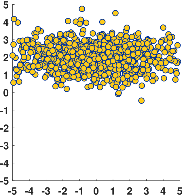
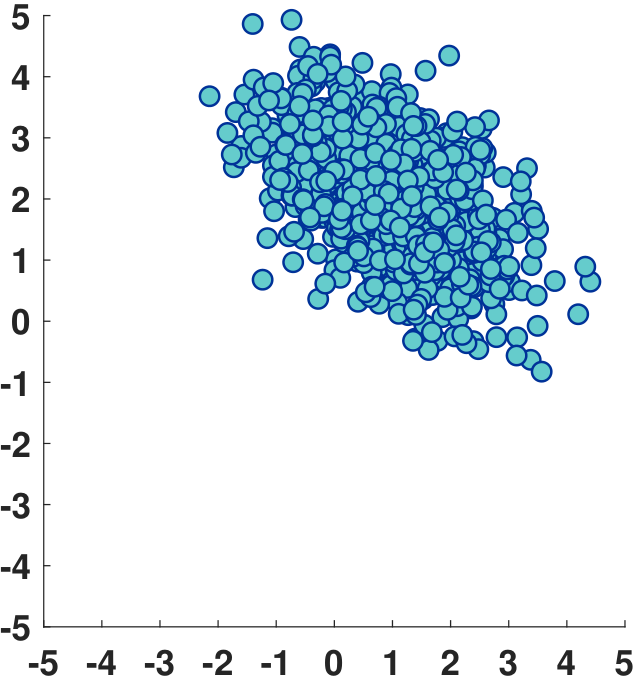
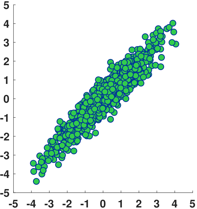
The Gaussian has different offsets and orientations for different choices of \(\vmu\) and \(\mSigma\). Figure 5.14 shows a few examples. Note that for \(\mSigma\) to be valid, \(\mSigma\) has to be “symmetric positive semi-definite”, the meaning of which will be explained shortly.

**Figure 5.14.** Visualization of 2D Gaussians with different means and covariances.

Generating random numbers from a multidimensional Gaussian can be done by calling built-in commands. In MATLAB, we use mvnrnd. In Python, we have a similar command.

MATLAB

% MATLAB code to generate random numbers from multivariate Gaussian
    mu    = [0 0];
    Sigma = [.25 .3; .3 1];
    X     = mvnrnd(mu,Sigma,100);

Python

# Python code to generate random numbers from multivariate Gaussian
    import numpy as np
    import scipy.stats as stats
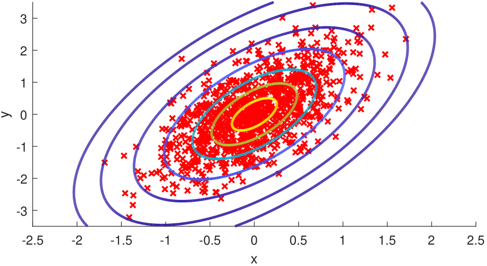
    X = stats.multivariate_normal.rvs([0,0],[[0.25,0.3],[0.3,1.0]],100)

To display the data points and overlay with the contour, we can use MATLAB commands such as contour. The resulting plot looks like the one shown in Figure 5.15. In Python the corresponding command is plt.contour. To set up the plotting environment we use the commands np.meshgrid. The grid points are used to evaluate the PDF values, thus giving us the contour.

MATLAB

% MATLAB code: Overlay random numbers with the Gaussian contour.
    X  = mvnrnd([0 0],[.25 .3; .3 1],1000);
    x1 = -2.5:.01:2.5;
    x2 = -3.5:.01:3.5;
    [X1,X2] = meshgrid(x1,x2);
    F = mvnpdf([X1(:) X2(:)],[0 0],[.25 .3; .3 1]);
    F = reshape(F,length(x2),length(x1));
    figure(1);
    scatter(x(:,1),x(:,2),'rx', 'LineWidth', 1.5); hold on;
    contour(x1,x2,F,[.001 .01 .05:.1:.95 .99 .999], 'LineWidth', 2);

Python

# Python code: Overlay random numbers with the Gaussian contour.
    import numpy as np
    import scipy.stats as stats
    import matplotlib.pyplot as plt
    X = stats.multivariate_normal.rvs([0,0],[[0.25,0.3],[0.3,1.0]],1000)
    x1 = np.arange(-2.5, 2.5, 0.01)
    x2 = np.arange(-3.5, 3.5, 0.01)
    X1, X2 = np.meshgrid(x1,x2)
    Xpos = np.empty(X1.shape + (2,))
    Xpos[:,:,0] = X1
    Xpos[:,:,1] = X2
    F = stats.multivariate_normal.pdf(Xpos,[0,0],[[0.25,0.3],[0.3,1.0]])
    plt.scatter(X[:,0],X[:,1])
    plt.contour(x1,x2,F)

**Figure 5.15.** 1000 random numbers drawn from a 2D Gaussian, overlaid with the contour plot.