Sum of Two Random Variables
One typical problem we encounter in engineering is to determine the PDF of the sum of two random variables \(X\) and \(Y\), i.e., \(X+Y\). Such a problem arises naturally when we want to evaluate the average of many random variables, e.g., the sample mean of a collection of data points. This section will discuss a general principle for determining the PDF of a sum of two random variables.
5.5.1Intuition through convolution
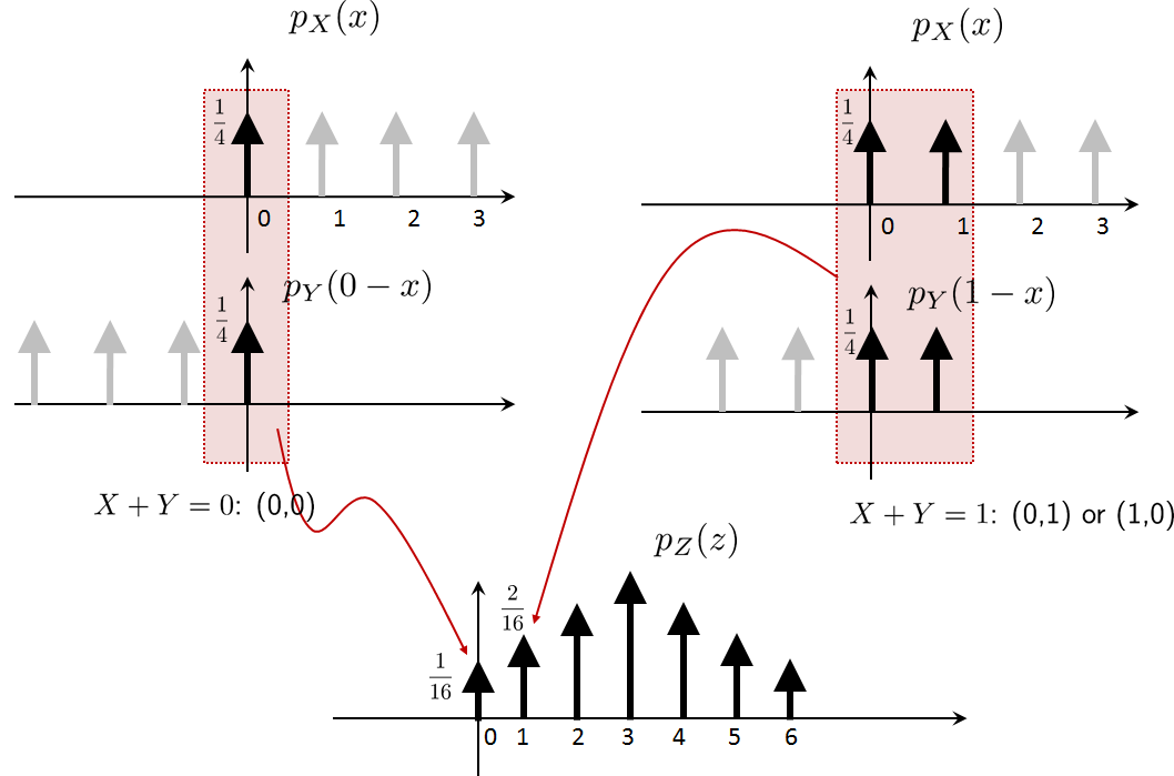
First, consider two random variables, \(X\) and \(Y\), both discrete uniform random variables in the range of \(0,1,2,3\). That is, \(p_X(x) = p_Y(y) = [1/4, 1/4, 1/4, 1/4]\). Since this is such a simple problem we can enumerate all the possible cases of the sum \(Z = X+Y\). The resulting probabilities are shown in the following table.
| \(Z = X+Y\) | Cases, written in terms of (X, Y) | Probability |
| 0 | (0,0) | 1/16 |
| 1 | (0,1), (1,0) | 2/16 |
| 2 | (1,1), (2,0), (0,2) | 3/16 |
| 3 | (3,0), (2,1), (1,2), (0,3) | 4/16 |
| 4 | (3,1), (2,2), (1,3) | 3/16 |
| 5 | (3,2), (2,3) | 2/16 |
| 6 | (3,3) | 1/16 |
Clearly, the PMF of \(Z\) is not \(f_Z(z) = f_X(x) + f_Y(y)\). (Caution! Do not write this.) The PMF of \(Z\) looks like a triangle distribution. How can we get to this triangle distribution from two uniform distributions? The key is the idea of convolution. Let us start with the PMF of \(X\), which is \(p_X(x)\). Let us also flip \(p_Y(y)\) over the \(y\)-axis. As we shift the flipped \(p_Y\), we multiply and add the PMF values as shown in Figure 5.11. This gives us
Now, if we shift towards the right by 1, we have
By continuing our argument, you can see that we will obtain the same PMF as the one shown in the table.
5.5.2Main result
We can show that for any arbitrary random variable \(X\) and \(Y\), the sum \(Z = X+Y\) has a distribution that is the convolution of two individual PDFs.
Let \(X\) and \(Y\) be two independent random variables with PDFs \(f_X(x)\) and \(f_Y(y)\) respectively. Let \(Z = X+Y\). The PDF of \(Z\) is given by
where “\(\ast\)” denotes the convolution.
Proof. We begin by analyzing the CDF of \(Z\). The CDF of \(Z\) is
We now draw a picture to illustrate the line under which we want to integrate. As shown in Figure 5.12, the equation \(X+Y\le z\) defines a straight line in the \(xy\) plane. You can think of it as \(Y \le -X + z\), so that the slope is \(-1\) and the \(y\)-intercept is \(z\).
Now, shall we take the upper half of the triangle or the lower half? Since the equation is \(Y \le -X + z\), a value of \(Y\) has to be less than that of the line. Another easy way to check is to assume \(z > 0\) so that we have a positive \(y\)-intercept. Then we check where the origin \((0,0)\) belongs. In this case, if \(z > 0\), the origin \((0,0)\) will satisfy the equation \(Y \le -X + z\), and so it must be included. Thus, we conclude that the area is below the line.
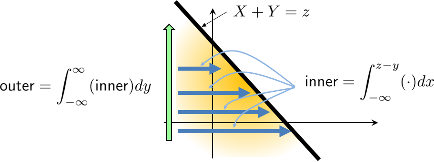
Once we have determined the area to be integrated, we can write down the integration:
where the integration limits are just a rewrite of \(X+Y \le z\) (in this case, since we are integrating \(x\) first, we have \(X \le -Y + z\)). Then, by the fundamental theorem of calculus, we can show that
where “\(\ast\)” denotes the convolution.
■- sep0ex
- If you sum \(X\) and \(Y\), the resulting PDF is the convolution of \(f_X\) and \(f_Y\).
- E.g., convolving two uniform random variables gives you a triangle PDF.
5.5.3Sum of common distributions
Let \(X_1 \sim \text{Poisson}(\lambda_1)\) and \(X_2 \sim \text{Poisson}(\lambda_2)\). Then
Proof. Let us apply the convolution principle.
where the last step is based on the binomial identity \(\sum_{\ell=0}^k {k \choose \ell} a^{\ell}b^{k-\ell} = (a+b)^k\).
■Let \(X_1\) and \(X_2\) be two Gaussian random variables such that $$X_1 \sim \text{Gaussian}(\mu_1,\sigma_1^2) \;\quad\text{and}\quad\; X_2 \sim \text{Gaussian}(\mu_2,\sigma_2^2).$$ Then
Proof. Let us apply the convolution principle by defining \(Z = X_1 + X_2\). Then,
We now complete the square:
Substituting these into the integral, we can show that
Therefore, we have shown that the resulting distribution is a Gaussian with mean \(\mu_1+\mu_2\) and variance \(\sigma_1^2+\sigma_2^2\).
■Let \(X\) and \(Y\) be independent, and let
Find the PDF of \(Z = X+Y\).
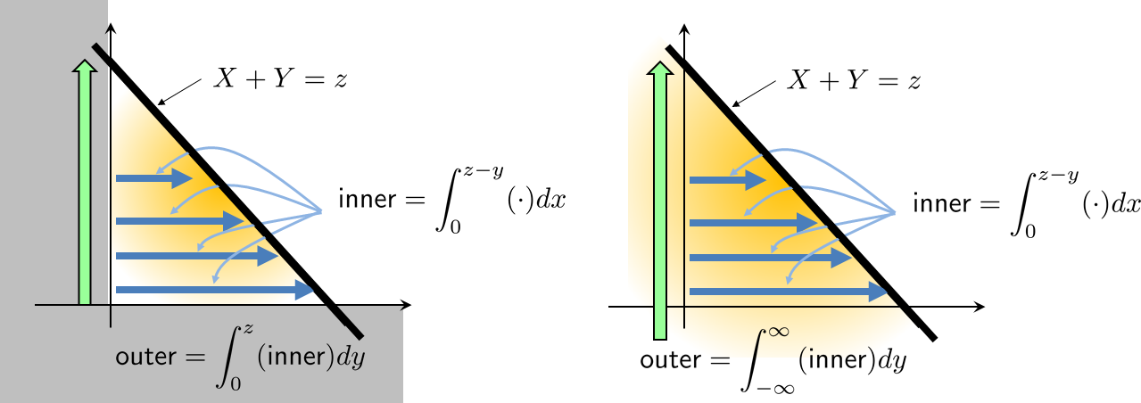
Using the results derived above, we see that
where the upper limit \(z\) came from the fact that \(x \ge 0\). Therefore, since \(Z = X + Y\), we must have \(Z - Y = X \ge 0\) and so \(Z \ge Y\). This is portrayed graphically in Figure 5.13. Substituting the PDFs into the integration yields
For \(z < 0\), \(f_Z(z) = 0\).
The functions of two random variables are not limited to summation. The following example illustrates the case of the product of two random variables.
Let \(X\) and \(Y\) be two independent random variables such that
Let \(Z = XY\). Find \(f_Z(z)\).
The CDF of \(Z\) can be evaluated as
Taking the derivative yields
where (a) holds by the fundamental theorem of calculus. The upper and lower limit of this integration can be determined by noting that
which implies that \(z \le y\). Since \(y \le 1\), we have that \(z \le y \le 1\). Therefore, the PDF is
For \(z<0\), \(f_Z(z) = 0\).
Closing remark. For some random variables, summing two i.i.d. copies remains the same random variable (but with different parameters). For other random variables, summing two i.i.d. copies gives a different random variable. Table 5.1 summarizes some of the most commonly used random variable pairs.
| \(X_1\) | \(X_2\) | Sum \(X_1 + X_2\) |
| \(\text{Bernoulli}(p)\) | \(\text{Bernoulli}(p)\) | \(\text{Binomial}(2,p)\) |
| \(\text{Binomial}(n,p)\) | \(\text{Binomial}(m,p)\) | \(\text{Binomial}(m+n,p)\) |
| \(\text{Poisson}(\lambda_1)\) | \(\text{Poisson}(\lambda_2)\) | \(\text{Poisson}(\lambda_1+\lambda_2)\) |
| \(\text{Exponential}(\lambda)\) | \(\text{Exponential}(\lambda)\) | \(\text{Erlang}(2,\lambda)\) |
| \(\text{Gaussian}(\mu_1,\sigma_1^2)\) | \(\text{Gaussian}(\mu_2,\sigma_2^2)\) | \(\text{Gaussian}(\mu_1+\mu_2,\sigma_1^2+\sigma_2^2)\) |