eBook › Chapter 5 · Joint Distributions

Section 5.4

Conditional Expectation

5.4.1Definition

When dealing with two dependent random variables, at times we would like to determine the expectation of a random variable when the second random variable takes a particular state. The conditional expectation is a formal way of doing so.

Definition 5.18

The conditional expectation of \(X\) given \(Y = y\) is

\E[X \,|\, Y = y] = \sum_{x} x p_{X|Y}(x|y)

for discrete random variables, and

\E[X \,|\, Y = y] = \int_{-\infty}^{\infty} x f_{X|Y}(x|y)\;dx

for continuous random variables.

There are two points to note here. First, the expectation of \(\E[X \,|\, Y = y]\) is taken with respect to \(f_{X|Y}(x|y)\). We assume that the random variable \(Y\) is already fixed at the state \(Y = y\). Thus, the only source of randomness is \(X\). Secondly, since the expectation \(\E[X \,|\, Y = y]\) has eliminated the randomness of \(X\), the resulting function is in \(y\).

0ex What is conditional expectation?

sep0ex
\(\E[X|Y=y]\) is the expectation using \(f_{X|Y}(x|y)\).
The integration is taken w.r.t. \(x\), because \(Y = y\) is given and fixed.

5.4.2The law of total expectation

Theorem 5.9

The law of total expectation states that

\E[X] = \sum_y \E[X|Y = y] p_Y(y), \quad\mbox{or}\quad \E[X] = \int_{-\infty}^{\infty} \E[X|Y = y] f_Y(y) \;dy.

Proof. We will prove the discrete case only, as the continuous case can be proved by replacing summation with integration.

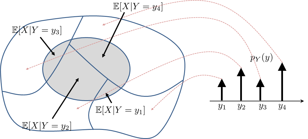
\begin{aligned} \E[X] &= \sum_{x} x p_X(x) = \sum_x x \left(\sum_{y} p_{X,Y}(x,y) \right) \\ &= \sum_x \sum_y x p_{X|Y}(x|y)p_Y(y) \\ &= \sum_y \left(\sum_x x p_{X|Y}(x|y)\right) p_Y(y) = \sum_y \E[X|Y=y] p_Y(y). \end{aligned}

■

Figure 5.10 illustrates the idea behind the proof. Essentially, we decompose the expectation \(\E[X]\) into “subexpectations” \(\E[X|Y = y]\). The probability of each subexpectation is \(p_Y(y)\). By summing the subexpectation multiplied by \(p_Y(y)\), we obtain the overall expectation.

0ex What is the law of total expectation?

sep0ex
The law of total expectation is a decomposition rule.
It decomposes \(\E[X]\) into smaller/easier conditional expectations.

This law can also be written in a more compact form.

Corollary 5.1

Let \(X\) and \(Y\) be two random variables. Then

\E[X] = \E_Y \left[ \E_{X|Y}[X|Y] \right].

Proof. The previous theorem states that \(\E[X] = \sum_y \E[X|Y = y] p_Y(y)\). If we treat \(\E[X|Y = y]\) as a function of \(y\), for instance \(h(y)\), then

\begin{aligned} \E[X] = \sum_y \E[X|Y = y] p_Y(y) = \sum_y h(y) p_Y(y) = \E[h(Y)] = \E \left[ \E[X|Y] \right]. \end{aligned}

■

Example 5.21

Suppose there are two classes of cars. Let \(X\) be the speed of a car and \(C\) be the class. When \(C = 1\), we know that \(X \sim \text{Gaussian}(\mu_1,\sigma_1^2)\). We know that \(\Pb[C = 1] = p\). When \(C = 2\), \(X \sim \text{Gaussian}(\mu_2,\sigma_2^2)\). Also, \(\Pb[C = 2] = 1-p\). If you see a car on the freeway, what is its average speed?

Solution

The problem has given us everything we need. In particular, we know that the conditional PDFs are:

\begin{aligned} f_{X|C}(x\,|\,1) &= \frac{1}{\sqrt{2\pi \sigma_1^2}} \exp\left\{-\frac{(x-\mu_1)^2}{2\sigma_1^2}\right\},\\ f_{X|C}(x\,|\,2) &= \frac{1}{\sqrt{2\pi \sigma_2^2}} \exp\left\{-\frac{(x-\mu_2)^2}{2\sigma_2^2}\right\}. \end{aligned}

Therefore, conditioned on \(C\), we have two expectations:

\begin{aligned} \E[X\,|\,C = 1] &= \int_{-\infty}^{\infty} x \, f_{X|C}(x\,|\,1) \;dx = \mu_1,\\ \E[X\,|\,C = 2] &= \int_{-\infty}^{\infty} x \, f_{X|C}(x\,|\,2) \;dx = \mu_2. \end{aligned}

The overall expectation \(\E[X]\) is

\begin{aligned} \E[X] %&= \sum_{c=1}^{2} \E[X|C = c] p_C(c)\\ &= \E[X\,|\,C = 1] \Pb[C = 1] + \E[X\,|\,C = 2] \Pb[C = 2]\\ &= p\mu_1 + (1-p)\mu_2. \end{aligned}

Practice Exercise 5.9

Consider a joint PMF given by the following table. Find \(\E[X|Y = 10^2]\) and \(\E[X|Y = 10^4]\).

\(Y\)	\(10^4\)	0	0	\(\frac{1}{12}\)	\(\frac{1}{18}\)	\(\frac{1}{36}\)
	\(10^2\)	\(\frac{5}{12}\)	\(\frac{5}{18}\)	\(\frac{5}{36}\)	0	0
		0.01	0.1	1	10	100
				\(X\)

Solution

To find the conditional expectation, we first need to know the conditional PMF.

\begin{aligned} p_{X|Y}(x|10^2) &= \begin{bmatrix}\frac{1}{2} & \frac{1}{3} & \frac{1}{6} & 0 & 0\end{bmatrix},\\ p_{X|Y}(x|10^4) &= \begin{bmatrix}0 & 0 & \frac{1}{2} & \frac{1}{3} & \frac{1}{6} \end{bmatrix}. \end{aligned}

Therefore, the conditional expectations are

\begin{aligned} \E[X\,|\,Y = 10^2] &= (10^{-2})\left(\frac{1}{2}\right) + (10^{-1})\left(\frac{1}{3}\right) + (1)\left(\frac{1}{6}\right) \\ &= \frac{123}{600},\\ \E[X\,|\,Y = 10^4] &= (1)\left(\frac{1}{2}\right) + (10)\left(\frac{1}{3}\right) + (100)\left(\frac{1}{6}\right) \\ &= \frac{123}{6}. \end{aligned}

From the conditional expectations we can also find \(\E[X]\):

\begin{aligned} \E[X] &= \E[X\,|\,Y = 10^2]p_Y(10^2) \\ &\qquad + \E[X\,|\,Y = 10^4]p_Y(10^4) \\ &= \left(\frac{123}{600}\right)\left(\frac{5}{6}\right) + \left(\frac{123}{6}\right)\left(\frac{1}{6}\right) \\ &= 3.5875. \end{aligned}

Example 5.22

Consider two random variables \(X\) and \(Y\). The random variable \(X\) is Gaussian-distributed with \(X \sim \text{Gaussian}(\mu,\sigma^2)\). The random variable \(Y\) has a conditional distribution \(Y|X \sim \text{Gaussian}(X,X^2)\). Find \(\E[Y]\).

Solution

The notation \(Y|X \sim \text{Gaussian}(X,X^2)\) means that given the variable \(X\), the other variable \(Y\) has a conditional distribution \(\text{Gaussian}(X,X^2)\). That is, the variable \(Y\) is a Gaussian with mean \(X\) and variance \(X^2\). How can the mean be a random variable \(X\) and the variance be another random variable \(X^2\)? Because \(X\) is the conditional variable. \(Y|X\) means that you have already chosen one state of \(X\). Given that particular state, the distribution of \(Y\) follows \(f_{Y|X}\). Therefore, for this problem, we know the PDFs:

\begin{aligned} f_X(x) &= \frac{1}{\sqrt{2\pi \sigma^2}} \exp\left\{-\frac{(x-\mu)^2}{2\sigma^2}\right\}, \\ f_{Y|X}(y|x) &= \frac{1}{\sqrt{2\pi x^2}} \exp\left\{-\frac{(y-x)^2}{2x^2}\right\}. \end{aligned}

The conditional expectation of \(Y\) given \(X\) is

\begin{aligned} \E[Y|X = x] &= \int_{-\infty}^{\infty} y \frac{1}{\sqrt{2\pi x^2}} \exp\left\{-\frac{(y-x)^2}{2x^2}\right\} \;dy \\ &= \E[\text{Gaussian}(x,x^2)] = x. \end{aligned}

The last equality holds because we are computing the expectation of a Gaussian random variable with mean \(x\). Finally, applying the law of total expectation, we can show that

\begin{aligned} \E[Y] &= \int_{-\infty}^{\infty} \E[Y|X = x]f_X(x) \;dx \\ &= \int_{-\infty}^{\infty} x \frac{1}{\sqrt{2\pi \sigma^2}} \exp\left\{-\frac{(x-\mu)^2}{2\sigma^2}\right\} \;dx \\ &= \E[\text{Gaussian}(\mu,\sigma^2)] = \mu, \end{aligned}

where the last equality is based on the fact that it is the mean of a Gaussian.

Practice Exercise 5.10

Find \(\E[\sin(X+Y)]\), if \(X \sim \text{Gaussian}(0,1)\), and \(Y \,|\, X \sim \mbox{Uniform}[x-\pi,x+\pi]\).

Solution

We know that the conditional density is

f_{Y|X}(y|x) = \frac{1}{2\pi}, \qquad x - \pi \le y \le x+\pi.

Therefore, we can compute the conditional expectation

\begin{aligned} \E[\sin(X+Y)|X=x] &= \int_{x-\pi}^{x+\pi} \sin(x+y) f_{Y|X}(y|x)\;dy \\ &= \frac{1}{2\pi} \underset{=0}{\underbrace{\int_{x-\pi}^{x+\pi} \sin(x+y) \;dy }} = 0. \end{aligned}

Hence, the overall expectation is

\begin{aligned} \E[\sin(X+Y)] = \int_{-\infty}^{\infty} \underset{=0}{\underbrace{\E[\sin(X+Y)|X=x]}} \frac{1}{\sqrt{2\pi}}e^{-\frac{x^2}{2}} \;dx = 0. \end{aligned}