Principal-Component Analysis

We have studied the covariance matrix \(\mSigma\) in some depth. It has many other uses besides transforming Gaussian random variables, and in this section we present one of them, called the principal-component analysis (PCA). PCA is a widely used tool for dimension reduction. Instead of using \(N\) features to describe a data point, PCA allows us to use the leading \(p\) principal components to describe the same data point. In many problems in machine learning, this makes the learning task easier and the inference task more efficient.

5.8.1The main idea: Eigendecomposition

PCA can be summarized in one sentence:

This is a condensed summary of PCA: It is just the eigendecomposition of the covariance. However, before we discuss the computational procedure, we will explain why we would want to perform the eigendecomposition of the covariance matrix.

Consider a set of data points \(\{\vx^{(1)},\ldots,\vx^{(N)}\}\), where each \(\vx^{(n)} \in \R^d\) is a \(d\)-dimensional vector. The dimension \(d\) is often high. For example, if we have an image of size \(1024 \times 1024 \times 3\), then \(d =\) 3,145,728 — not a huge number, but enough to make you feel dizzy. The goal of PCA is to find a low-dimensional representation in \(\R^p\) where \(p \ll d\). If we can find this low-dimensional representation, we can represent the \(d\)-dimensional input using only \(p\) coefficients. Since \(p \ll d\), we can “compress” the data by using a compact representation. In modern data science, such a dimension reduction scheme is useful for handling large-scale datasets.

Mathematically, we define a set of basis vectors \(\vv_1,\ldots,\vv_p\), where each \(\vv_i \in \R^d\). Our goal is to approximate an input data point \(\vx^{(n)} \in \R^d\) by these basis vectors:

where \(\{\alpha_i\}_{i=1}^p\) are called the representation coefficients. The representation described by this equation is a linear representation. Linear representation is extremely common in practice. For example, a data point \(\vx^{(n)} = [7,1,4]^T\) can be represented as

Therefore, the 3-dimensional input \(\vx^{(n)}\) can now be represented by two coefficients \(\alpha_1 = 3\) and \(\alpha_2 = 4\). This is called dimensionality reduction.

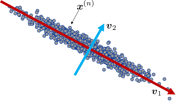
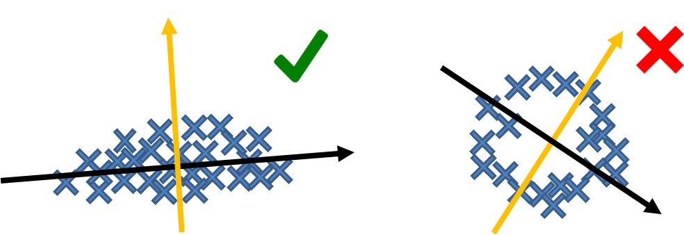
Pictorially, if we have already determined the basis vectors, we can compute the coefficients for every data point in the dataset. However, not all basis vectors are good. As illustrated in Figure 5.21, an elongated dataset will be of the greatest benefit if the basis vectors are oriented according to the data geometry. If we can find such basis vectors, then the data points will have a large coefficient and a small coefficient, corresponding to the major and the minor axes. Dimensionality reduction can thus be achieved by, for example, only keeping the larger coefficients.

The challenge here is that, given the dataset \(\{\vx^{(1)},\ldots,\vx^{(N)}\}\), we need to determine both the basis vectors \(\{\vv_i\}_{i=1}^p\) and the coefficients \(\{\alpha_i\}_{i=1}^p\). Fortunately, this can be formulated as an eigendecomposition problem.

To see how this problem can be thus formulated, we consider the simplest case as illustrated in Figure 5.21, where we want to find the leading principal component. That is, we find \((\alpha,\vv)\) such that \(\vx \approx \alpha\vv\). This amounts to solving the optimization problem

The notation “argmin” means the argument that minimizes the function. The equation says that we find the \((\alpha,\vv)\) that minimizes the distance between \(\vx\) and \(\alpha\vv\). The constraint \(\|\vv\|_2 = 1\) limits the search to within a unit circle; otherwise our solution will not be unique.

Solving the optimization problem is not difficult. If we take the derivative w.r.t. \(\alpha\) and set it to zero, we have that

Substituting \(\alpha = \vx^T\vv\) into the objective function again, we show that

Let us pause for a second. We have shown that if we have one data point \(\vx\), the leading principal component \(\vv\) can be determined by maximizing \(\vv^T\vx \vx^T\vv\). What have we gained? We have transformed the original optimization, which contains two variables \((\vv,\alpha)\), to a new optimization that contains one variable \(\vv\). Thus if we know how to solve the one-variable problem we are done.

However, there is one more issue we need to address before we discuss how to solve the problem. The issue is that the formulation is about one data sample, not the entire dataset. To include all the samples, we need to assume that \(\vx\) is a realization of a random vector \(\mX\). Then the above optimization can be formulated in the expectation sense as

where \(\mSigma \bydef \E[\mX\mX^T]\). (Here we assume that \(\mX\) is zero-mean, i.e., \(\E[\mX] = 0\). If it is not, then we can subtract the mean by considering \(\argmax{\|\vv\|_2 = 1} \; \vv^T \E\bigg\{(\mX-\vmu) (\mX-\vmu)^T\bigg\} \vv\).) Therefore, if we can maximize \(\vv^T\mSigma\vv\) we will be able to determine the principal component.

Now comes the main result. The following theorem shows that the maximization is equivalent to eigendecomposition. The proof requires Lagrange multipliers, which are beyond the scope of this book.

We want to prove that the solution to the problem

is the eigenvector of the matrix \(\mSigma\). To show that, we first write down the Lagrangian:

Taking the derivative w.r.t. \(\vv\) and setting to zero yields

This is equivalent to \(\mSigma\vv = \lambda\vv\). So if \(\mSigma = \mU\mS\mU^T\), then by letting \(\vv = \vu_i\) and \(\lambda = s_i\) we can satisfy the condition since \(\mSigma\vu_i = \mU\mS\mU^T\vu_i = \mU\mS\ve_i = s_i\vu_i\).

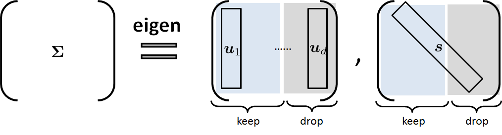
This theorem can be extended to the second (and other) principal components of the covariance matrix. In fact, given the covariance matrix \(\mSigma\) we can follow the procedure outlined in Figure 5.22 to determine the principal components. The eigendecomposition of a \(d \times d\) matrix \(\mSigma\) will give us a \(d \times d\) eigenvector matrix \(\mU\) and an eigenvalue matrix \(\mS\). To keep the \(p\) leading eigenvectors, we truncate the \(\mU\) matrix to only use the first \(p\) eigenvectors. Here, we assume that the eigenvectors are ordered according to the magnitude of the eigenvalues, from large to small.

In practice, if we are given a dataset \(\{\vx^{(1)},\ldots,\vx^{(N)}\}\), we can first estimate the covariance matrix \(\mSigma\) by

where \(\widehat{\vmu} = \frac{1}{N}\sum_{n=1}^N \vx^{(n)}\) is the mean vector. Afterwards, we can compute the eigendecomposition of \(\widehat{\mSigma}\) by

On a computer, the principal components are obtained through eigendecomposition. A MATLAB example and a Python example are shown below. We explicitly show the two principal components in this example. The magnitudes of these two vectors are determined by the eigenvalues diag(s).

% MATLAB code to perform the principal-component analysis
    x = mvnrnd([0,0],[2 -1.9; -1.9 2],1000);
    covX = cov(x);
    [U,S] = eig(covX);
    u(:,1) % Principal components
    u(:,2) % Principal components

# Python code to perform the principal-component analysis
    import numpy as np
    x  = np.random.multivariate_normal([1,-2],[[3,-0.5],[-0.5,1]],1000)
    covX = np.cov(x,rowvar=False)
    S, U = np.linalg.eig(covX)
    print(U)

Example 5.27

Suppose we have a dataset containing \(N = 1000\) samples, drawn from an unknown distribution. The first few samples are

$$\begin{aligned} \vx_1 = \begin{bmatrix} 0.5254 \\ -0.6930 \end{bmatrix}, \quad \vx_2 = \begin{bmatrix} -0.4040 \\ 0.3724 \end{bmatrix}, \quad \ldots \; , \quad \vx_{1000} = \begin{bmatrix} 1.4165 \\ -1.5463 \end{bmatrix}. \end{aligned}$$

We can compute the mean and covariance using MATLAB commands mean and cov. This will return us

$$\widehat{\vmu} = \begin{bmatrix} 0.0561 \\ -0.0303 \end{bmatrix} \quad\text{and}\quad \widehat{\mSigma} = \begin{bmatrix} 2.0460 & -1.9394\\ -1.9394 & 2.0426 \end{bmatrix}.$$

Applying eigendecomposition on \(\widehat{\mSigma}\), we show that

$$\begin{aligned} &[\mU,\mS] = \text{eig}(\widehat{\mSigma}),\\ & \qquad \Longrightarrow \mU = \begin{bmatrix} -0.7068 & -0.7074\\ -0.7074 & 0.7068 \end{bmatrix} \quad \text{and} \quad \mS = \begin{bmatrix} 0.1049 & 0\\ 0 & 3.9837 \end{bmatrix}. \end{aligned}$$

Therefore, we have obtained two principal components

$$\vu_1 = \begin{bmatrix} -0.7068 \\ -0.7074 \end{bmatrix} \qquad\text{and}\qquad \vu_2 = \begin{bmatrix} -0.7074 \\ 0.7068 \end{bmatrix}.$$

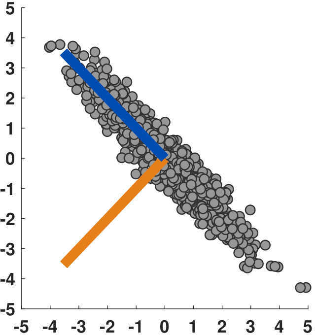
As seen in the figure below, these two principal components make sense. The vector \(\vu_1\) is the orange line and is the minor axis. The vector \(\vu_2\) is the blue line and is the major axis. Again, the ordering of the vectors is determined by the eigenvalues. Since \(\vu_2\) has a larger eigenvalue (=3.9837), it is the leading principal component.

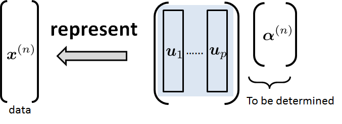
Why do we call our method principal component analysis? The analysis part comes from the fact that we can compress a data vector \(\vx^{(n)}\) from a high dimension \(d\) to a low dimension \(p\). Defining \(\mU_p = [\vu_1,\ldots,\vu_p]\), a matrix containing the \(p\) leading eigenvectors of the matrix \(\mU\), we solve the inverse problem:

where the goal is to determine the coefficient vector \(\valpha^{(n)} \in \R^p\). Since \(\mU_p\) is an orthonormal matrix (i.e., \(\mU_p^T\mU_p = \mI\)), it follows that

as illustrated in Figure 5.24. Hence,

This equation is a projection operation that projects a data point \(\vx^{(n)}\) onto the space spanned by the \(p\) leading principal components. Repeating the procedure for all the data points \(\vx^{(1)},\ldots,\vx^{(N)}\) in the dataset, we have compressed the dataset.

5.8.2The eigenface problem

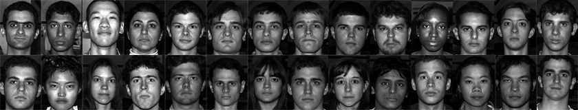
As a concrete example of PCA, we consider a computer vision problem called the eigenface problem. In 2001, researchers at Yale University published the Yale Database, and a few years later they extended it to a larger one (http://vision.ucsd.edu/ leekc/ExtYaleDatabase/ExtYaleB.html). The dataset, now known as the Yale Face Dataset, contains 16,128 images of 28 human subjects under nine poses and 64 illumination conditions. The sizes of the images are \(d = 168\times192 =\) 32,256 pixels. Treating these \(N =\)16,128 images as vectors in \(\R^{32,256\times 1}\), we have 16,128 of these vectors. Let us call them \(\{\vx^{(1)},\ldots,\vx^{(N)}\}\).

Following the procedure we described above, we estimate the covariance matrix by computing

where \(\vmuhat = \E[\mX] \approx \frac{1}{N}\sum_{n=1}^N \vx^{(n)}\) is the mean vector. Note that the size of \(\vmuhat\) is 32,256\(\times\)1 and the size of \(\mSigmahat\) is 32,256 \(\times\) 32,256.

Once we obtain an estimate of the covariance matrix, we can perform an eigendecomposition to get

The columns of \(\mU\), i.e., \(\{\vu_i\}_{i=1}^d\), are the eigenvectors of \(\mSigmahat\). These eigenvectors are the basis of a testing face image.

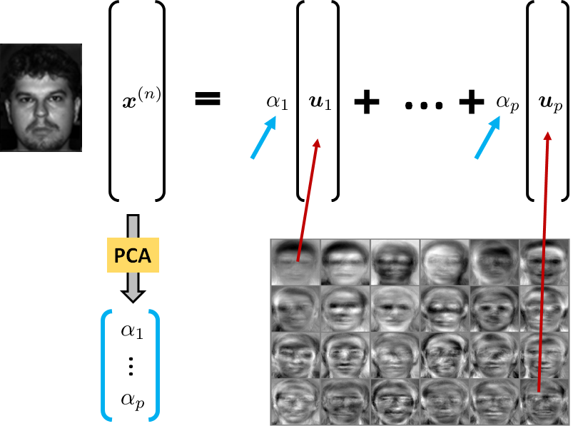
With the basis vectors \(\vu_1,\ldots,\vu_p\) we can project every image in the dataset using a low-dimensional representation. Specifically, for an image \(\vx\) we compute the coefficients

or more compactly \(\valpha = \mU^T\vx\). Note that the dimension of \(\vx\) is \(d \times 1\) (which in our case is \(d=\) 32,256), and the dimensions of \(\valpha\) can be as few as \(p = 100\). Therefore, we are using a \(100\)-dimensional vector to represent a 32,256-dimensional data point. This is a huge dimensionality reduction.

The process repeats for all the samples \(\vx^{(1)}, \ldots, \vx^{(N)}\). This gives us a collection of representation coefficients \(\valpha^{(1)},\ldots,\valpha^{(N)}\), where each \(\valpha^{(n)}\) is \(100\)-dimensional (see Figure 5.26). Notice that the basis vectors \(\vu_i\) appear more or less like “face images,” but they are the features of the faces. PCA says that a real face can be written as a linear combination of these basis vectors.

5.8.3What cannot be analyzed by PCA?

PCA is a dimension reduction tool. It compresses a raw data vector \(\vx \in \R^d\) into a smaller feature vector \(\valpha \in \R^p\). The advantage is that the downstream learning problems are much easier because \(p \ll d\). For example, classification using \(\valpha\) is more efficient than classification using \(\vx\) since there is very little information loss from \(\vx\) to \(\valpha\).

There are three limitations of PCA:

• sep0ex
• PCA fails when the raw data are not orthogonal. The basis vectors \(\vu_i\) returned by PCA are orthogonal, meaning that \(\vu_i^T\vu_j = 0\) as long as \(i \not= j\). As a result, if the data intrinsically have this orthogonality property, then PCA will work very well. However, if the data live in a space such as a donut shape as illustrated in Figure 5.27, then PCA will fail. Here, by failure, we mean that \(p\) is not much smaller than \(d\). To handle datasets behaving like Figure 5.27, we need advanced tools. One of these is the kernel-PCA. The idea is to apply a nonlinear transformation to the data before you run PCA.

• sep0ex
• Basis vectors returned by PCA are not interpretable. A temptation with PCA is to think that the basis vectors \(\vu_i\) offer meaningful information because they are the “principal components”. However, since PCA is the eigendecomposition of the covariance matrix, which is purely a mathematical operation, there is no guarantee that the basis vectors contain any semantic meaning. If we look at the basis vectors shown in Figure 5.26, there is almost no information one can draw. Therefore, in the data-science literature, alternative methods such as non-negative matrix factorization and the more recent deep neural network embedding are more attractive because the feature vectors sometimes (not always) have meanings.
• PCA does not return you the most influential “component”. Imagine that you are analyzing medical data for research on a disease, in which each data vector \(\vx^{(n)}\) contains height, weight, BMI, blood pressure, etc. When you run PCA on the dataset, you will obtain some “principal components”. However, these principal components will likely have everything, e.g., the height entry of the principal component will have some values, the weight will have some values, etc. If you have found a principal component, it does not mean that you have identified the leading risk factor of the disease. If you want to identify the leading risk factor of the disease, e.g., whether the height or weight is more important, you need to resort to advanced tools such as variable selection or the LASSO type of regression analysis (see Chapter 7).

Closing remark. PCAs are powerful computational tools based on the simplest concept of covariance matrices because, as our derivation showed, covariance matrices encode the “variation” of the data. Therefore, by finding a vector that aligns with the maximum variation of the data, we can find the principal component.

% ========== YC's Bookmark ========