Transformation of Multidimensional Gaussians

As we have seen in Figure 5.14, the shape and orientation of a multidimensional Gaussian are determined by the mean vector \(\vmu\) and the covariance matrix \(\mSigma\). This means that if we can somehow transform the mean vector and the covariance matrix, we will get another Gaussian. A few practical questions are:

• sep0ex
• How do we shift and rotate a Gaussian random variable?
• If we have an arbitrary Gaussian, how do we go back to zero-mean unit-variance Gaussian?
• How do we generate random vectors according to a predefined Gaussian?

These questions come up frequently in data analysis. Answering the first two questions will help us transform Gaussians back and forth, while answering the last question will help us with generating random samples.

5.7.1Linear transformation of mean and covariance

Suppose we have an arbitrary (not necessarily a Gaussian) vector \(\mX = [X_1,\ldots,X_N]^T\) with mean \(\vmu_X\) and covariance \(\mSigma_X\). Entries of \(\mX\) are not necessarily independent. Let \(\mA \in \R^{N \times N}\) be a transformation, and let \(\mY = \mA\mX\). That is,

Then we can show the following result.

What if we shift the random vector by defining \(\mY = \mX + \vb\)? We state the following result without proof (try proving it as an exercise).

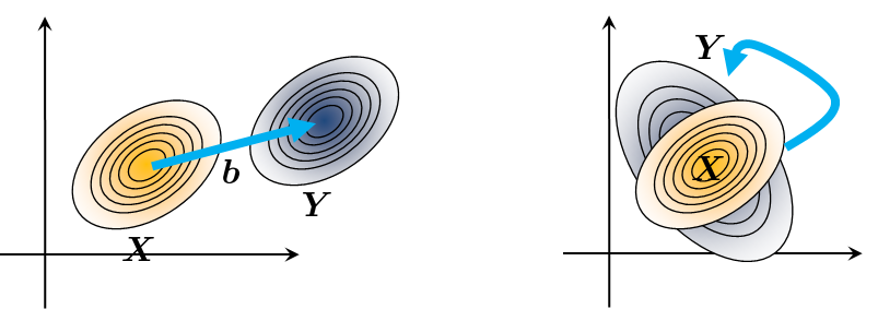
For a Gaussian random vector, the linear transformations either shift the Gaussian or rotate the Gaussian, as shown in Figure 5.16:

• sep0ex
• If we add \(\vb\) to \(\mX\), the resulting operation is a translation.
• If we multiply \(\mA\) by \(\mX\), then the resulting operation is a rotation and scaling.

5.7.2Eigenvalues and eigenvectors

As our next step, we need to understand eigendecomposition. You can easily find relevant background in any undergraduate linear algebra textbook. Here we provide a summary for completeness.

When applying a matrix \(\mA\) to a vector \(\vx\), a typical engineering question is: what \(\vx\) would be invariant to \(\mA\)? Or in other words, for what \(\vx\) can we make sure that \(\mA \vx = \lambda \vx\), for some scalar \(\lambda\)? If we can find such a vector \(\vx\), we say that \(\vx\) is the eigenvector of \(\mA\). Eigenvectors are useful for seeking principal components of datasets or finding efficient signal representations. They are defined as follows:

An \(N \times N\) matrix has at most \(N\) eigenvalues. Therefore, the above equation can be generalized to

for \(i = 1,\ldots,N\), or more compactly as \(\mA\mU = \mU\mLambda\). The eigenvalues \(\lambda_1,\ldots,\lambda_N\) are not necessarily distinct. There are matrices with identical eigenvalues, the identity matrix being a trivial example. However, not all square matrices are diagonalizable. For example, the matrix \(\begin{bmatrix}0 & 1\\0 & 0\end{bmatrix}\) has a repeated eigenvalue 0 but only one independent eigenvector, so it cannot be diagonalized.

There are a number of equivalent conditions for \(\lambda\) to be an eigenvalue:

• There exists \(\vu \not= 0\) such that \(\mA\vu = \lambda\vu\);
• There exists \(\vu \not= 0\) such that \((\mA-\lambda\mI)\vu = \vzero\);
• \((\mA-\lambda\mI)\) is not invertible;
• \(\det(\mA-\lambda\mI) = 0\).

We are mostly interested in symmetric matrices. If \(\mA\) is symmetric, then all the eigenvalues are real, and the following result holds.

We call such a decomposition the eigendecomposition. In MATLAB, we can compute the eigenvalues of a matrix by using the eig command. In Python, the corresponding command is np.linalg.eig. Note that in our demonstration below we symmetrize the matrix. This step is needed, for otherwise the eigenvalues will contain complex numbers.

% MATLAB Code to perform eigendecomposition
    A = randn(100,100);
    A = (A + A')/2;     % symmetrize because A is not symmetric
    [U,S] = eig(A);     % eigendecomposition
    s = diag(S);        % extract eigenvalue

# Python Code to perform eigendecomposition
    import numpy as np
    A = np.random.randn(100,100)
    A = (A + np.transpose(A))/2
    S, U = np.linalg.eig(A)
    s = np.diag(S)

The condition that \(\mU^T\mU = \mI\) is the result of an orthonormal matrix. Equivalently, \(\vu_i^T\vu_j = 1\) if \(i = j\) and \(\vu_i^T\vu_j = 0\) if \(i \not= j\). Since \(\{\vu_i\}_{i=1}^{N}\) is orthonormal, it can serve as a basis of any vector in \(\R^N\):

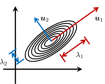
where \(\alpha_j = \vu_j^T\vx\) is called the basis coefficient. Basis vectors are useful in that they can provide alternative representations of a vector. The geometry of the joint Gaussian is determined by its eigenvalues and eigenvectors. Consider the eigendecomposition of \(\mSigma\):

for some unitary matrix \(\mU\) and diagonal matrix \(\mLambda\). The columns of \(\mU\) are called the eigenvectors, and the entries of \(\mLambda\) are called the eigenvalues. Since \(\mSigma\) is symmetric, all \(\lambda_i\)'s are real. In addition, since \(\mSigma\) is positive semi-definite, all \(\lambda_i\)'s are non-negative. Accordingly, the volume defined by the multidimensional Gaussian is always a convex object, e.g., an ellipse in 2D or an ellipsoid in 3D.

The orientation of the axes is defined by the column vectors \(\vu_i\). In the case of \(d=2\), the major axis is defined by \(\vu_1\) and the minor axis is defined by \(\vu_2\). The corresponding radii of each axis are specified by the eigenvalues \(\lambda_1\) and \(\lambda_2\). Figure 5.17 provides an illustration.

5.7.3Covariance matrices are always positive semi-definite

Now that we understand eigendecomposition, what can we do with it? Here is one practical problem. Given a matrix \(\mSigma\), how do you know that it is a valid covariance matrix? For example, if we give you a singular matrix, then \(\mSigma^{-1}\) may not exist. Checking the validity of \(\mSigma\) requires the concept of positive semi-definite.

Given a matrix \(\mA \in \R^{N \times N}\), it is important to check the positive semi-definiteness of \(\mA\). There are two practical scenarios where we need positive semi-definiteness. (1) If we are estimating the covariance matrix \(\mSigma\) from a dataset, we need to ensure that \(\mSigma = \E[(\mX-\vmu)(\mX-\vmu)^T]\) is positive semi-definite because all covariance matrices are positive semi-definite. Otherwise, the matrix we estimate is not a legitimate covariance matrix. (2) If we solve an optimization problem involving a function \(f(\vx) = \vx^T\mA\vx\), then having \(\mA\) being positive semi-definite, we can guarantee that the problem is convex. Convex problems ensure that a local minimum is also global, and convex problems can be solved efficiently using known algorithms.

Using eigendecomposition, it is not difficult to show that positive semi-definiteness is equivalent to having non-negative eigenvalues.

The following corollary shows that if \(\mA \in \R^{N \times N}\) is positive definite, it must be invertible. Being invertible also means that the columns of \(\mA\) are linearly independent.

The next theorem tells us that the covariance matrix is always positive semi-definite.

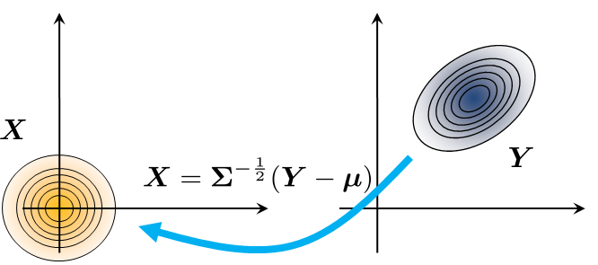
5.7.4Gaussian whitening

Besides checking positive semi-definiteness, another typical problem we encounter is how to generate random samples according to some Gaussian distributions.

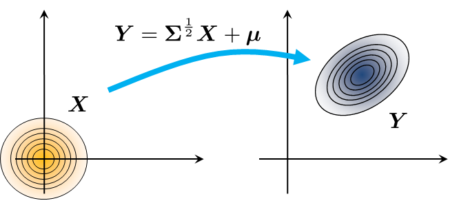
From \(\text{Gaussian}(\vzero,\mI)\) to \(\text{Gaussian}(\vmu,\mSigma)\). If we are given zero-mean unit-variance Gaussian \(\mX \sim \text{Gaussian}(\vzero,\mI)\), how do we generate \(\mY \sim \text{Gaussian}(\vmu,\mSigma)\) from \(\mX\)?

The idea is to define a transformation

where \(\mSigma^{\frac{1}{2}} = \mU\mLambda^{\frac{1}{2}}\mU^T\). Then the mean of \(\mY\) is

and the covariance matrix is

Therefore, the two steps for doing this Gaussian whitening are:

• sep0ex
• Step 1: Generate samples \(\{\vx_1,\ldots,\vx_N\}\) that are distributed according to \(\text{Gaussian}(\vzero,\mI)\).

• Step 2: Define \(\vy_n\) where

  $$\vy_n = \mSigma^{\frac{1}{2}}\vx_n + \vmu.$$

These two steps are portrayed in Figure 5.18.

Example 5.26

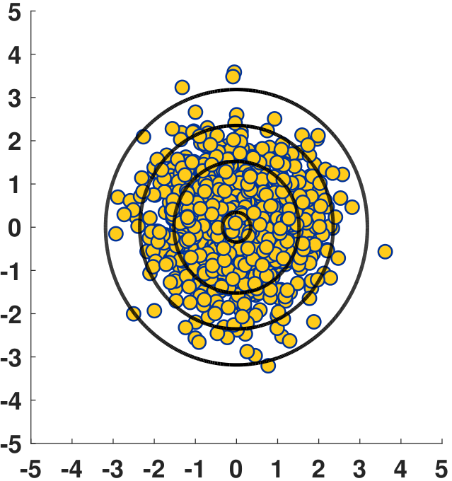
Consider a set of \(N = 1000\) i.i.d. \(\text{Gaussian}(\vzero,\mI)\) data points as shown in Figure 5.19, for example,

$$\begin{aligned} \vx_1 = \begin{bmatrix} 0.5377\\ 1.8399 \end{bmatrix} , \qquad \vx_2 = \begin{bmatrix} -2.2588\\ 0.8622 \end{bmatrix} , \qquad \ldots \; , \qquad \vx_{1000} = \begin{bmatrix} 0.3188\\ -1.3077 \end{bmatrix}. \end{aligned}$$

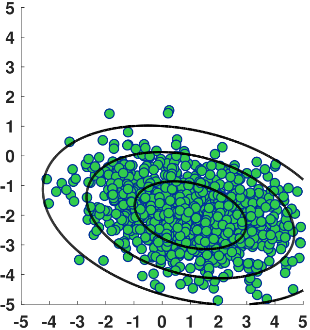
Transform these data points so that the new distribution is a Gaussian with

$$\vmu = \begin{bmatrix} 1\\ -2 \end{bmatrix} \quad\mbox{and}\quad \mSigma = \begin{bmatrix} 3 & -0.5 \\ -0.5 & 1 \end{bmatrix}.$$

Solution. To perform the transformation, we first perform eigendecomposition of \(\mSigma = \mU\mLambda\mU^T\). Then \(\mSigma^{\frac{1}{2}} = \mU\mLambda^{\frac{1}{2}}\mU^T\). For our problem, we compute

$$\mSigma^{\frac{1}{2}} = \begin{bmatrix} 1.722 & -0.1848 \\ -0.1848 & 0.9828 \end{bmatrix}.$$

Multiplying this matrix to yield \(\vy_n = \mSigma^{\frac{1}{2}}\vx_n + \vmu\), we obtain

$$\begin{aligned} \vy_1 = \begin{bmatrix} 1.5870\\ -0.2971 \end{bmatrix} , \qquad \vy_2 = \begin{bmatrix} -3.0495\\ -0.7351 \end{bmatrix} , \qquad \ldots \; , \qquad \vy_{1000} = \begin{bmatrix} 1.7907\\ -3.3441 \end{bmatrix}. \end{aligned}$$

In MATLAB, the above whitening procedure can be realized using the following commands.

% MATLAB code to perform the whitening
    x     = mvnrnd([0,0],[1 0; 0 1],1000);
    Sigma = [3 -0.5; -0.5 1];
    mu    = [1; -2];
    y     = Sigma^(0.5)*x' + mu;

The Python implementation is similar, although one needs to be careful with the more complicated syntax. For example, Sigma^(0.5) in MATLAB does the eigen-based matrix power automatically, whereas in Python we need to call a specific built-in command fractional_matrix_power. In MATLAB, broadcasting a vector to a matrix can be recognized. In Python, we need to call repmat explicitly to control the shape of the mean vectors.

# Python code to perform the whitening
    import numpy as np
    import scipy.stats as stats
    from scipy.linalg import fractional_matrix_power
    
    x      = np.random.multivariate_normal([0,0],[[1,0],[0,1]],1000)
    mu     = np.array([1,-2])
    Sigma  = np.array([[3, -0.5],[-0.5, 1]])
    Sigma2 = fractional_matrix_power(Sigma,0.5)
    y      = np.dot(Sigma2, x.T) + np.matlib.repmat(mu,1000,1).T

From \(\text{Gaussian}(\vmu,\mSigma)\) to \(\text{Gaussian}(\vzero,\mI)\). The reverse direction can be done as follows. Supposing that we have \(\mY \sim \text{Gaussian}(\vmu,\mSigma)\), we define

Then

The covariance is

The following theorem summarizes this result.

Thus the two steps of doing this reversed Gaussian whitening are:

• sep0ex
• Step 1: Assuming that \(\vy_1,\ldots,\vy_N\) are distributed as \(\text{Gaussian}(\vmu,\mSigma)\), estimate \(\vmu\) and \(\mSigma\).

• Step 2: Define \(\vx_n\) where

  $$\vx_n = \mSigma^{-\frac{1}{2}}(\vy_n - \vmu).$$

These two steps are shown pictorially in Figure 5.20.

In practice, if we are given \(\{\vy_n\}_{n=1}^N\), we need to estimate \(\vmu\) and \(\mSigma\). The estimations are quite straightforward.

On computers, these can be obtained using the command mean and cov. Once we have calculated \(\widehat{\vmu}\) and \(\widehat{\mSigma}\), we can define \(\vx_n\) as

On computers, the codes for the whitening procedure that uses the estimated mean and covariance are shown below.

% MATLAB code to perform whitening
    y    = mvnrnd([1; -2],[3 -0.5; -0.5 1],100);
    mY   = mean(y);
    covY = cov(y);
    x    = covY^(-0.5)*(y-mY)';

# Python code to perform whitening
    import numpy as np
    import scipy.stats as stats
    from scipy.linalg import fractional_matrix_power
    y  = np.random.multivariate_normal([1,-2],[[3,-0.5],[-0.5,1]],100)
    mY = np.mean(y,axis=0)
    covY  = np.cov(y,rowvar=False)
    covY2 = fractional_matrix_power(covY,-0.5)
    x     = np.dot(covY2, (y-np.matlib.repmat(mY,100,1)).T)