eBook › Chapter 5 · Joint Distributions

Section 5.3

Conditional PMF and PDF

Whenever we have a pair of random variables $X$ and $Y$ that are correlated, we can define their conditional distributions, which quantify the probability of $X = x$ given $Y = y$. In this section, we discuss the concepts of conditional PMF and PDF.

5.3.1Conditional PMF

We start by defining the conditional PMF for a pair of discrete random variables.

Definition 5.14

Let $X$ and $Y$ be two discrete random variables. The conditional PMF of $X$ given $Y$ is

p_{X|Y}(x|y) = \frac{p_{X,Y}(x,y)}{p_Y(y)}.

The simplest way to understand this is to view $p_{X|Y}(x|y)$ as $\Pb[X = x \,|\, Y = y]$. That is, given that $Y = y$, what is the probability for $X = x$? To see why this perspective makes sense, let us recall the definition of a conditional probability:

\begin{aligned} p_{X|Y}(x|y) &= \frac{p_{X,Y}(x,y)}{p_Y(y)} \\ &= \frac{\Pb[X = x \, \cap \, Y = y]}{\Pb[Y = y]} = \Pb[X = x \,|\, Y = y]. \end{aligned}

As we can see, the last two equalities are essentially the definitions of conditional probability and the joint PMF.

How should we understand the notation $p_{X|Y}(x|y)$? Is it a one-variable function in $x$ or a two-variable function in $(x,y)$? What does $p_{X|Y}(x|y)$ tell us? To answer these questions, let us first try to understand the randomness exhibited in a conditional PMF. In $p_{X|Y}(x|y)$, the random variable $Y$ is fixed to a specific value $Y = y$. Therefore, there is nothing random about $Y$. All the possibilities of $Y$ have already been taken care of by the denominator $p_Y(y)$. Only the variable $x$ in $p_{X|Y}(x|y)$ has randomness. What do we mean by “fixed at a value $Y = y$”? Consider the following example.

Example 5.16

Suppose there are two coins. Let

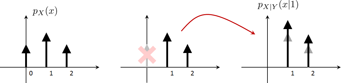
\begin{aligned} X &= \text{the sum of the values of two coins},\\ Y &= \text{the value of the first coin}. \end{aligned}

Clearly, $X$ has 3 states: 0, 1, 2, and $Y$ has two states: either 0 or 1. When we say $p_{X|Y}(x|1)$, we refer to the probability mass function of $X$ when fixing $Y = 1$. If we do not impose this condition, the probability mass of $X$ is simple: $$p_X(x) = \left[\frac{1}{4}, \frac{1}{2}, \frac{1}{4}\right].$$ However, if we include the conditioning, then

\begin{aligned} p_{X|Y}(x|1) &= \frac{p_{X,Y}(x,1)}{p_{Y}(1)} \\ &= \frac{\left[0, \frac{1}{4}, \frac{1}{4}\right]}{\frac{1}{2}} = \left[0, \frac{1}{2}, \frac{1}{2}\right]. \end{aligned}

To put this in plain words, when $Y = 1$, there is no way for $X$ to take the state 0. The chance for $X$ to take the state 1 is $1/2$ because only $(1,0)$ can give $X = 1$ when the first coin is fixed at 1. The chance for $X$ to take the state 2 is $1/2$ because it has to be $(1,1)$ in order to give $X = 2$. Therefore, when we say “conditioned on $Y = 1$”, we mean that we limit our observations to cases where $Y = 1$. Since $Y$ is already fixed at $Y = 1$, there is nothing random about $Y$. The only variable is $X$. This example is illustrated in Figure 5.9.

**Figure 5.9.** Suppose $X$ is the sum of two coins with PMF $0.25, 0.5, 0.25$. Let $Y$ be the first coin. When $X$ is unconditioned, the PMF is just $[0.25, 0.5, 0.25]$. When $X$ is conditioned on $Y = 1$, then “$X = 0$” cannot happen. Therefore, the resulting PMF $p_{X|Y}(x|1)$ only has two states. After normalization we obtain the conditional PMF $[0, 0.5, 0.5]$.

Since $Y$ is already fixed at a particular value $Y = y$, $p_{X|Y}(x|y)$ is a probability mass function of $x$ (we want to emphasize again that it is $x$ and not $y$). So $p_{X|Y}(x|y)$ is a one-variable function in $x$. It is not the same as the usual PMF $p_X(x)$. $p_{X|Y}(x|y)$ is conditioned on $Y = y$. For example, $p_{X|Y}(x|1)$ is the PMF of $X$ restricted to the condition that $Y = 1$. In fact, it follows that

\begin{aligned} \sum_{x \in \Omega_X} p_{X|Y}(x|y) &= \sum_{x \in \Omega_X} \frac{p_{X,Y}(x,y)}{p_Y(y)} \\ &= \frac{\sum_{x \in \Omega_X} p_{X,Y}(x,y)}{p_Y(y)} = \frac{p_Y(y)}{p_Y(y)} = 1, \end{aligned}

and this tells us that $p_{X|Y}(x|y)$ is a legitimate probability mass of $X$. If we sum over the $y$'s instead, then we will hit a bump: $$\sum_{y \in \Omega_Y} p_{X|Y}(x|y) = \sum_{y \in \Omega_Y} \frac{p_{X,Y}(x,y)}{p_Y(y)} \not= 1.$$ Therefore, while $p_{X|Y}(x|y)$ is a legitimate probability mass function of $X$, it is not a probability mass function of $Y$.

Example 5.17

Consider a joint PMF given in the following table. Find the conditional PMF $p_{X|Y}(x|1)$ and the marginal PMF $p_X(x)$.

		Y=
	1	2	3	4
X = 1	$\frac{1}{20}$	$\frac{1}{20}$	$\frac{1}{20}$	$\frac{0}{20}$
2	$\frac{1}{20}$	$\frac{2}{20}$	$\frac{3}{20}$	$\frac{1}{20}$
3	$\frac{1}{20}$	$\frac{2}{20}$	$\frac{3}{20}$	$\frac{1}{20}$
4	$\frac{0}{20}$	$\frac{1}{20}$	$\frac{1}{20}$	$\frac{1}{20}$

Solution

To find the marginal PMF, we sum over all the $y$'s for every $x$:

\begin{aligned} x = 1: &\quad p_{X}(1) = \sum_{y=1}^{4} p_{X,Y}(1,y) = \frac{1}{20} + \frac{1}{20} + \frac{1}{20} + \frac{0}{20} = \frac{3}{20},\\ x = 2: &\quad p_{X}(2) = \sum_{y=1}^{4} p_{X,Y}(2,y) = \frac{1}{20} + \frac{2}{20} + \frac{3}{20} + \frac{1}{20} = \frac{7}{20},\\ x = 3: &\quad p_{X}(3) = \sum_{y=1}^{4} p_{X,Y}(3,y) = \frac{1}{20} + \frac{2}{20} + \frac{3}{20} + \frac{1}{20} = \frac{7}{20},\\ x = 4: &\quad p_{X}(4) = \sum_{y=1}^{4} p_{X,Y}(4,y) = \frac{0}{20} + \frac{1}{20} + \frac{1}{20} + \frac{1}{20} = \frac{3}{20}. \end{aligned}

Hence, the marginal PMF is

\begin{aligned} p_{X}(x) = \begin{bmatrix} \frac{3}{20} & \frac{7}{20} & \frac{7}{20} & \frac{3}{20}\end{bmatrix}. \end{aligned}

The conditional PMF $p_{X|Y}(x|1)$ is

\begin{aligned} p_{X|Y}(x|1) &= \frac{p_{X,Y}(x,1)}{p_Y(1)} = \frac{\begin{bmatrix} \frac{1}{20} & \frac{1}{20} & \frac{1}{20} & \frac{0}{20}\end{bmatrix}}{\frac{3}{20}} = \begin{bmatrix} \frac{1}{3} & \frac{1}{3} & \frac{1}{3} & 0\end{bmatrix}. \end{aligned}

Practice Exercise 5.7

Consider two random variables $X$ and $Y$ defined as follows.

\begin{aligned} Y = \begin{cases} 10^2, &\quad \mbox{with prob } 5/6,\\ 10^4, &\quad \mbox{with prob } 1/6. \end{cases} \quad X = \begin{cases} 10^{-4}Y, &\quad \mbox{with prob } 1/2,\\ 10^{-3}Y, &\quad \mbox{with prob } 1/3,\\ 10^{-2}Y, &\quad \mbox{with prob } 1/6. \end{cases} \end{aligned}

Find $p_{X|Y}(x|y)$, $p_X(x)$ and $p_{X,Y}(x,y)$.

Solution

Since $Y$ takes two different states, we can enumerate $Y = 10^2$ and $Y = 10^4$. This gives us

\begin{aligned} p_{X|Y}(x|10^2) &= \begin{cases} 1/2, &\quad\mbox{if } x = 0.01,\\ 1/3, &\quad\mbox{if } x = 0.1,\\ 1/6, &\quad\mbox{if } x = 1. \end{cases}\\ p_{X|Y}(x|10^4) &= \begin{cases} 1/2, &\quad\mbox{if } x = 1,\\ 1/3, &\quad\mbox{if } x = 10,\\ 1/6, &\quad\mbox{if } x = 100. \end{cases} \end{aligned}

The joint PMF $p_{X,Y}(x,y)$ is

\begin{aligned} p_{X,Y}(x,10^2) &= p_{X|Y}(x|10^2)p_Y(10^2) = \begin{cases} \left(\frac{1}{2}\right)\left(\frac{5}{6}\right), &\quad x = 0.01,\\ \left(\frac{1}{3}\right)\left(\frac{5}{6}\right), &\quad x = 0.1,\\ \left(\frac{1}{6}\right)\left(\frac{5}{6}\right), &\quad x = 1. \end{cases} \end{aligned}

\begin{aligned} p_{X,Y}(x,10^4) &= p_{X|Y}(x|10^4)p_Y(10^4) = \begin{cases} \left(\frac{1}{2}\right)\left(\frac{1}{6}\right), &\quad x = 1,\\ \left(\frac{1}{3}\right)\left(\frac{1}{6}\right), &\quad x = 10,\\ \left(\frac{1}{6}\right)\left(\frac{1}{6}\right), &\quad x = 100. \end{cases} \end{aligned}

Therefore, the joint PMF is given by the following table.

$10^4$	0	0	$\frac{1}{12}$	$\frac{1}{18}$	$\frac{1}{36}$
$10^2$	$\frac{5}{12}$	$\frac{5}{18}$	$\frac{5}{36}$	0	0
	0.01	0.1	1	10	100

The marginal PMF $p_X(x)$ is thus

\begin{aligned} p_X(x) &= \sum_{y} p_{X,Y}(x,y) \\ &= \begin{bmatrix} \frac{5}{12} & \frac{5}{18} & \frac{2}{9} & \frac{1}{18} & \frac{1}{36} \end{bmatrix}. \end{aligned}

In the previous two examples, what is the probability $\Pb[X \in A \,|\, Y = y]$ or the probability $\Pb[X \in A]$ for some events $A$? The answers are given by the following theorem.

Theorem 5.7

Let $X$ and $Y$ be two discrete random variables. Let $A$ be an event.

\Pb[ X \in A \,|\, Y = y] = \sum_{x \in A} p_{X|Y}(x|y)

and

\begin{aligned} \Pb[ X \in A] &= \sum_{x \in A} \sum_{y \in \Omega_Y} p_{X|Y}(x|y)p_Y(y) = \sum_{y \in \Omega_Y} \Pb[X \in A \,|\, Y = y]p_Y(y). \end{aligned}

Proof. The first statement is based on the fact that if $A$ contains a finite number of elements, then $\Pb[X \in A]$ is equivalent to the sum $\sum_{x \in A}\Pb[X = x]$. Thus,

\begin{aligned} \Pb[ X \in A \,|\, Y = y] &= \frac{\Pb[X \in A \cap Y = y]}{\Pb[Y = y]} \\ &= \frac{\sum_{x \in A} \Pb[X = x \cap Y = y]}{\Pb[Y = y]}\\ &= \sum_{x \in A} p_{X|Y}(x|y). \end{aligned}

The second statement holds because the inner summation $\sum_{y \in \Omega_Y} p_{X|Y}(x|y)p_Y(y)$ is just the marginal PMF $p_X(x)$. Thus the outer summation yields the probability.

■

Example 5.18

Let us follow up on Example 5.17. What is the probability that $\Pb[X > 2|Y= 1]$? What is the probability that $\Pb[X > 2]$?

Solution

Since the problem asks about the conditional probability, we know that it can be computed by using the conditional PMF. This gives us

\begin{aligned} \Pb[X > 2 | Y = 1] &= \sum_{x > 2} p_{X|Y}(x|1) \\ &= \cancel{p_{X|Y}(1|1)} + \cancel{p_{X|Y}(2|1)} + \underset{\frac{1}{3}}{\underbrace{p_{X|Y}(3|1)}} + \underset{0}{\underbrace{p_{X|Y}(4|1)}} = \frac{1}{3}. \end{aligned}

The other probability is

\begin{aligned} \Pb[X > 2] &= \sum_{x > 2} p_{X}(x) = \cancel{p_X(1)} + \cancel{p_X(2)} + \underset{\frac{7}{20}}{\underbrace{p_X(3)}} + \underset{\frac{3}{20}}{\underbrace{p_X(4)}} = \frac{10}{20}. \end{aligned}

What is the rule of thumb for conditional distribution?

sep0ex
The PMF/PDF should match with the probability you are finding.
If you want to find the conditional probability $\Pb[X \in A|Y=y]$, use the conditional PMF $p_{X|Y}(x|y)$.
If you want to find the probability $\Pb[X \in A]$, use the marginal PMF $p_{X}(x)$.

Finally, we define the conditional CDF for discrete random variables.

Definition 5.15

Let $X$ and $Y$ be discrete random variables. Then the conditional CDF of $X$ given $Y = y$ is

F_{X|Y}(x|y) = \Pb[X \le x \,|\, Y = y] = \sum_{x' \le x} p_{X|Y}(x'|y).

5.3.2Conditional PDF

We now discuss the conditioning of a continuous random variable.

Definition 5.16

Let $X$ and $Y$ be two continuous random variables. The conditional PDF of $X$ given $Y$ is

f_{X|Y}(x|y) = \frac{f_{X,Y}(x,y)}{f_Y(y)}.

Example 5.19

Let $X$ and $Y$ be two continuous random variables with a joint PDF

\begin{aligned} f_{X,Y}(x,y) = \begin{cases} 2e^{-x}e^{-y}, &\quad\quad 0 \le y \le x < \infty, \\ 0, &\quad\quad \mbox{otherwise}. \end{cases} \end{aligned}

Find the conditional PDFs $f_{X|Y}(x|y)$ and $f_{Y|X}(y|x)$.

Solution

We first find the marginal PDFs.

\begin{aligned} f_X(x) &= \int_{-\infty}^{\infty} f_{X,Y}(x,y) \;dy = \int_{0}^{x} 2e^{-x}e^{-y}\;dy = 2e^{-x}(1-e^{-x}),\\ f_Y(y) &= \int_{-\infty}^{\infty} f_{X,Y}(x,y) \;dx = \int_{y}^{\infty} 2e^{-x}e^{-y} \;dx = 2e^{-2y}. \end{aligned}

Thus, the conditional PDFs are

\begin{aligned} f_{X|Y}(x|y) &= \frac{f_{X,Y}(x,y)}{f_Y(y)} \\ &= \frac{2e^{-x}e^{-y}}{2e^{-2y}} = e^{-(x-y)}, \quad x\ge y,\\ f_{Y|X}(y|x) &= \frac{f_{X,Y}(x,y)}{f_X(x)} \\ &= \frac{2e^{-x}e^{-y}}{2e^{-x}(1-e^{-x})} = \frac{e^{-y}}{1-e^{-x}}, \quad 0 \le y < x. \end{aligned}

Where does the conditional PDF come from? We cannot duplicate the argument we used for the discrete case because the denominator of a conditional PMF becomes ${\Pb[Y = y] = 0}$ when $Y$ is continuous. To answer this question, we first define the conditional CDF for continuous random variables.

Definition 5.17

Let $X$ and $Y$ be continuous random variables. Then the conditional CDF of $X$ given $Y = y$ is

F_{X|Y}(x|y) = \frac{\int_{-\infty}^{x} f_{X,Y}(x',y)\;dx'}{f_Y(y)}.

Why should the conditional CDF of continuous random variable be defined in this way? One way to interpret $F_{X|Y}(x|y)$ is as the limiting perspective. We can define the conditional CDF as

\begin{aligned} F_{X|Y}(x|y) &= \lim_{h\rightarrow 0} \Pb(X \le x \,|\, y \le Y \le y+h) \\ &= \lim_{h\rightarrow 0} \frac{\Pb(X \le x \cap y \le Y \le y+h)}{\Pb[y \le Y \le y+h]}. \end{aligned}

With some calculations, we have that

\begin{aligned} \lim_{h\rightarrow 0} \frac{\Pb(X \le x \cap y \le Y \le y+h)}{\Pb[y \le Y \le y+h]} &= \lim_{h\rightarrow 0} \frac{\int_{-\infty}^{x}\int_{y}^{y+h} f_{X,Y}(x',y')\;dy' \;dx'}{\int_{y}^{y+h} f_{Y}(y')\;dy'} \\ &= \lim_{h\rightarrow 0} \frac{\int_{-\infty}^{x} f_{X,Y}(x',y') \;dx' \cdot h}{f_{Y}(y) \cdot h} \\ &= \frac{\int_{-\infty}^{x} f_{X,Y}(x',y') \;dx' }{f_{Y}(y)}. \end{aligned}

The key here is that the small step size $h$ in the numerator and the denominator will cancel each other out. Now, given the conditional CDF, we can verify the definition of the conditional PDF. It holds that

\begin{aligned} f_{X|Y}(x|y) &= \frac{d}{dx} F_{X|Y}(x|y) \\ &= \frac{d}{dx} \left\{\frac{\int_{-\infty}^{x} f_{X,Y}(x',y)\;dx'}{f_Y(y)}\right\} \overset{(a)}{=} \frac{f_{X,Y}(x,y)}{f_Y(y)}, \end{aligned}

where (a) follows from the fundamental theorem of calculus.

Just like the conditional PMF, we can calculate the probabilities using the conditional PDFs. In particular, if we evaluate the probability where $X \in A$ given that $Y$ takes a particular value $Y = y$, then we can integrate the conditional PDF $f_{X|Y}(x|y)$, with respect to $x$.

Theorem 5.8

Let $X$ and $Y$ be continuous random variables, and let $A$ be an event.

sep0ex
(i) $\Pb[X \in A \;|\; Y = y] = \int_{A} f_{X|Y}(x|y) \;dx$,
(ii) $\Pb[X \in A] = \int_{\Omega_Y} \Pb[X \in A \,|\, Y=y] f_Y(y) \;dy$.

Example 5.20

Let $X$ be a random bit such that

\begin{aligned} X = \begin{cases} +1, & \mbox{with prob } 1/2, \\ -1, & \mbox{with prob } 1/2. \end{cases} \end{aligned}

Suppose that $X$ is transmitted over a noisy channel so that the observed signal is

\begin{aligned} Y = X + N, \end{aligned}

where $N \sim \text{Gaussian}(0,1)$ is the noise, which is independent of the signal $X$. Find the probabilities $\Pb[X = +1 \,|\, Y > 0]$ and $\Pb[X = -1 \,|\, Y > 0]$.

Solution

First, we know that

\begin{aligned} f_{Y|X}(y|+1) = \frac{1}{\sqrt{2\pi}} e^{-\frac{(y-1)^2}{2}} \qquad\text{and}\qquad f_{Y|X}(y|-1) = \frac{1}{\sqrt{2\pi}} e^{-\frac{(y+1)^2}{2}}. \end{aligned}

Therefore, integrating $y$ from $0$ to $\infty$ gives us

\begin{aligned} \Pb[Y > 0 \,|\, X = +1] &= \int_{0}^{\infty} \frac{1}{\sqrt{2\pi}} e^{-\frac{(y-1)^2}{2}} \;dy \\ &= 1-\int_{-\infty}^{0} \frac{1}{\sqrt{2\pi}} e^{-\frac{(y-1)^2}{2}} \;dy \\ &= 1-\Phi\left(\frac{0-1}{1}\right) = 1-\Phi(-1). \end{aligned}

Similarly, we have $\Pb[Y > 0 \,|\, X = -1] = 1-\Phi(+1)$. The probability we want to find is $\Pb[X = +1 \,|\, Y > 0]$, which can be determined using Bayes' theorem.

\begin{aligned} \Pb[X = +1 \,|\, Y > 0] &= \frac{\Pb[Y > 0 \,|\, X = +1]\Pb[X = +1]}{\Pb[Y > 0]}. \end{aligned}

The denominator can be found by using the law of total probability:

\begin{aligned} \Pb[Y > 0] &= \Pb[Y > 0 \,|\, X = +1]\Pb[X=+1] \\ &\quad + \Pb[Y > 0 \,|\, X = -1]\Pb[X = -1]\\ &= 1-\frac{1}{2}\left(\Phi(+1)+\Phi(-1)\right) \\ &= \frac{1}{2}, \end{aligned}

since $\Phi(+1)+\Phi(-1) = \Phi(+1)+1-\Phi(+1) = 1$. Therefore,

\begin{aligned} \Pb[X = +1 \,|\, Y > 0] &= 1-\Phi(-1) \\ &= 0.8413. \end{aligned}

The implication is that if $Y>0$, the probability $\Pb[X = +1 \,|\, Y > 0] = 0.8413$. The complement of this result gives $\Pb[X = -1 \,|\, Y > 0] = 1-0.8413 = 0.1587$.

Practice Exercise 5.8

Find $\Pb[Y > y]$, where $$X \sim \mathrm{Uniform}[1,2], \quad Y \,|\, X \sim \mathrm{Exponential}(x).$$

Solution

The tricky part of this problem is the tendency to confuse the two variables $X$ and $Y$. Once you understand their roles, the problem becomes easy. First notice that $Y \,|\, X \sim \mathrm{Exponential}(x)$ is a conditional distribution. It says that given $X = x$, the probability distribution of $Y$ is exponential, with the parameter $x$. Thus, we have that

f_{Y|X}(y|x) = x e^{-xy}.

Why? Recall that if $Y \sim \text{Exponential}(\lambda)$ then $f_Y(y) = \lambda e^{-\lambda y}$. Now if we replace $\lambda$ with $x$, we have $xe^{-xy}$. So the role of $x$ in this conditional density function is as a parameter.

Given this property, we can compute the conditional probability:

\begin{aligned} \Pb[Y > y \,|\, X = x] &= \int_{y}^{\infty} f_{Y|X}(y'|x) \;dy' \\ &= \int_{y}^{\infty} x e^{-xy'} \;dy' = \bigg[-e^{-xy'}\bigg]_{y'=y}^{\infty} = e^{-xy}. \end{aligned}

Finally, we can compute the marginal probability:

\begin{aligned} \Pb[Y > y] &= \int_{\Omega_X} \Pb[Y > y | X = x'] f_X(x') \;dx' \\ &= \int_{1}^{2} e^{-x'y} \;dx' = \bigg[-\frac{1}{y}e^{-x'y}\bigg]_{x'=1}^{x'=2} = \frac{1}{y}\left(e^{-y}-e^{-2y}\right). \end{aligned}

We can double-check this result by noting that the problem asks about the probability $\Pb[Y > y]$. Thus, the answer must be a function of $y$ but not of $x$.

		Y=
	1	2	3	4
X = 1	\(\frac{1}{20}\)	\(\frac{1}{20}\)	\(\frac{1}{20}\)	\(\frac{0}{20}\)
2	\(\frac{1}{20}\)	\(\frac{2}{20}\)	\(\frac{3}{20}\)	\(\frac{1}{20}\)
3	\(\frac{1}{20}\)	\(\frac{2}{20}\)	\(\frac{3}{20}\)	\(\frac{1}{20}\)
4	\(\frac{0}{20}\)	\(\frac{1}{20}\)	\(\frac{1}{20}\)	\(\frac{1}{20}\)

\(10^4\)	0	0	\(\frac{1}{12}\)	\(\frac{1}{18}\)	\(\frac{1}{36}\)
\(10^2\)	\(\frac{5}{12}\)	\(\frac{5}{18}\)	\(\frac{5}{36}\)	0	0
	0.01	0.1	1	10	100